ΑΙhub.org
An inferential perspective on federated learning
TL;DR: motivated to better understand the fundamental tradeoffs in federated learning, we present a probabilistic perspective that generalizes and improves upon federated optimization and enables a new class of efficient federated learning algorithms.
Thanks to deep learning, today we can train better machine learning models when given access to massive data. However, the standard, centralized training is impossible in many interesting use-cases—due to the associated data transfer and maintenance costs (most notably in video analytics), privacy concerns (e.g., in healthcare settings), or sensitivity of the proprietary data (e.g., in drug discovery). And yet, different parties that own even a small amount of data want to benefit from access to accurate models. This is where federated learning comes to the rescue!
Broadly, federated learning (FL) allows multiple data owners (or clients) to train shared models collaboratively under the orchestration of a central server without having to share raw data. Typically, FL proceeds in multiple rounds of communication between the server and the clients: the clients compute model updates on their local data and send them to the server which aggregates and applies these updates to the shared model. While gaining popularity very quickly, FL is a relatively new subfield with many open questions and unresolved challenges.
Here is one interesting conundrum driving our work:
Client-server communication is often too slow and expensive. To speed up training (often x10-100) we can make clients spend more time at each round on local training (e.g., do more local SGD steps), thereby reducing the total number of communication rounds. However, because of client data heterogeneity (natural in practice), it turns out that increasing the amount of local computation per round results in convergence to inferior models!
This phenomenon is illustrated below in Figure 1 on a toy convex problem, where we see that more local steps lead the classical federated averaging (FedAvg) algorithm to converge to points that are much further away from the global optimum. But why does this happen?
In this post, we will present a probabilistic perspective on federated learning that will help us better understand this phenomenon and design new FL algorithms that can utilize local computation much more efficiently, converging faster, to better optima.
The classical approach: FL as a distributed optimization problem
Federated learning was originally introduced as a new setting for distributed optimization with a few distinctive properties such as a massive number of distributed nodes (or clients), slow and expensive communication, and unbalanced and non-IID data scattered across the nodes. The main goal of FL is to approximate centralized training (the gold-standard) and converge to the same optimum as the centralized optimization would have, at the fastest rate possible.
Mathematically, FL is formulated as minimization of a linear combination of local objectives,  :
:
![\[\min_{\theta \in \mathbb{R}^d} \left\{F(\theta) := \sum_{i=1}^N q_i f_i(\theta) \right\}\]](https://aihub.org/wp-content/ql-cache/quicklatex.com-0d1509d5e9a0e19822318d45bf6411d0_l3.png "Rendered by QuickLaTeX.com")
where the weights  are usually set proportional to the sizes
  of the local datasets to make
  match the centralized training objective. So, how can we solve this optimization problem within a minimal number of communication rounds?
The trick is simple: at each round  , instead of asking clients to estimate and send gradients of their local objective functions (as done in conventional distributed optimization), let them optimize their objectives for multiple steps (or even epochs!) to obtain
  and send differences (or “deltas”) between the initial
  and updated states to the server as pseudo-gradients, which the server then averages, scales by a learning rate
  , and uses to update the model state:
![\[\theta^{t+1} = \theta^t + \alpha_t \sum_{i=1}^N q_i \Delta_i^t, \quad \text{where}\ \Delta_i^t := \theta^t - \theta_i^t\]](https://aihub.org/wp-content/ql-cache/quicklatex.com-4780ca4c4449526294ae4e39d1e60bf3_l3.png "Rendered by QuickLaTeX.com")
This approach, known as FedAvg or local SGD, allows clients to make more progress at each round. And since taking additional SGD steps locally is orders of magnitude faster than communicating with the server, the method converges much faster both in the number of rounds and in wall-clock time.
The problem (a.k.a. “client drift”): as we mentioned in the beginning, allowing multiple local SGD steps between client-server synchronization makes the algorithm converge to an inferior optimum in the non-IID setting (i.e., when clients have different data distributions) since the resulting pseudo-gradients turn out to be somehow biased compared to centralized training.
There are ways to overcome client drift using local regularization, carefully setting learning rate schedules, or using different control variate methods, but most of these mitigation strategies intentionally have to limit the optimization progress clients can make at each round.
Fundamentally, viewing FL as a distributed optimization problem runs into a tradeoff between the amount of local progress allowed and the quality of the final solution.
So, is there a way around this fundamental limitation?
An alternative approach: FL via posterior inference
Typically, client objectives  correspond to log-likelihoods of their local data. Therefore, statistically speaking, FL is solving a maximum likelihood estimation (MLE) problem. Instead of solving it using distributed optimization techniques, however, we can take a Bayesian approach: first, infer the posterior distribution,
  , then identify its mode which will be the solution.
Why is posterior inference better than optimization? Because any posterior can be exactly decomposed into a product of sub-posteriors:
![\[P(\theta \mid D) \propto \prod_{i=1}^N P(\theta \mid D_i)\]](https://aihub.org/wp-content/ql-cache/quicklatex.com-6af02623c6baa63619399762e147b4df_l3.png "Rendered by QuickLaTeX.com")
Thus, we are guaranteed to find the correct solution in three simple steps:
- Infer local sub-posteriors on each client and send their sufficient statistics to the server.
- Multiplicatively aggregate sub-posteriors on the server into the global posterior.
- Find and return the mode of the global posterior.
Wait, isn’t posterior inference intractable!? 
Indeed, there is a reason why posterior inference is not as popular as optimization: it is either intractable or often significantly more complex and computationally expensive. Moreover, posterior distributions rarely have closed form expressions and require various approximations.
For example, consider federated least squares regression, with quadratic local objectives:  In this case, the global posterior mode has a closed form expression:
![\[\theta^\star = \left( \sum_{i=1}^N q_i \Sigma_i^{-1} \right)^{-1} \left( \sum_{i=1}^N q_i \Sigma_i^{-1} \mu_i \right)\]](https://aihub.org/wp-content/ql-cache/quicklatex.com-f8ccb33902d32d767a88a238beed89a1_l3.png "Rendered by QuickLaTeX.com")
where  and
and  are the means and covariances of the local posteriors. Even though in this simple case the posterior is Gaussian and inference is technically tractable, computing
  requires inverting multiple matrices and communicating local means and covariances from the clients to the server. In comparison to FedAvg, which requires only
  computation and communication per round, posterior inference seems like a very bad idea…
Approximate inference FTW! 
Turns out that we can compute approximately using an elegant distributed inference algorithm which we call federated posterior averaging (or FedPA):
- On the server, we can compute iteratively over multiple rounds:
![\[\theta^{t+1} = \theta^t - \alpha_t \sum_{i=1}^N q_i \underbrace{\Sigma_i^{-1}\left( \theta^t - \mu_i \right)}_{:= \Delta_i^t}\]](https://aihub.org/wp-content/ql-cache/quicklatex.com-5068890ff1742561744ec7dbd1ee7dad_l3.png "Rendered by QuickLaTeX.com")
where
is the server learning rate. This procedure avoids the outer matrix inverse and requires clients to send to the server only some delta vectors instead of full covariance matrices. Also, the summation can be substituted with a stochastic approximation, i.e., only a subset of clients must participate in each round. Note how similar it is to FedAvg! - On the clients, we can compute
 very efficiently in two steps:
- Use stochastic gradient Markov chain Monte Carlo (SG-MCMC) to produce multiple approximate samples from the local posterior.
- Use an efficient dynamic programming procedure to compute the inverse covariance matrix multiplied by a vector in time and memory.
Note: in the case of arbitrary non-Gaussian likelihoods (which is the case for deep neural nets), FedPA essentially approximates the local and global posteriors with the best fitting Gaussians (a.k.a. the Laplace approximation).
What is the difference between FedAvg and FedPA? 
FedPA has the same computation and communication complexity as FedAvg. In fact, the algorithms differ only in how the client updates  are computed. Since FedAvg computes
  , we can also view it as an approximate posterior inference algorithm that estimates local covariances with identity matrices, which results in biased updates!
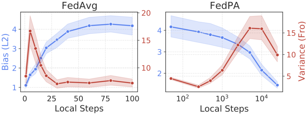
Figure 2 illustrates the difference between FedAvg and FedPA in terms of the bias and variance of updates they compute at each round as functions of the number of SGD steps:
- More local SGD steps increase the bias of FedAvg updates, leading the algorithm to converge to a point further away from the optimum.
- FedPA uses local SGD steps to produce more posterior samples, which improves the estimates of the local means and covariances and reduces the bias of model updates.
Does FedPA actually work in practice? 
The bias-variance tradeoff argument seems great in theory, but does it actually work in practice? First, let’s revisit our toy 2D example with 2 clients and quadratic objectives:
We see that not only is FedPA as fast as FedAvg initially but it also converges to a point that is significantly closer to the global optimum. At the end of convergence, FedPA exhibits some oscillations that could be further eliminated by increasing the number of local posterior samples.
Next, let’s compare FedPA with FedAvg head-to-head on realistic and challenging benchmarks, such as the federated CIFAR100 and StackOverflow datasets:
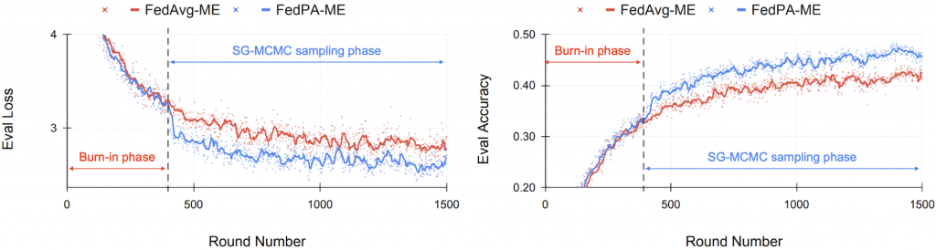
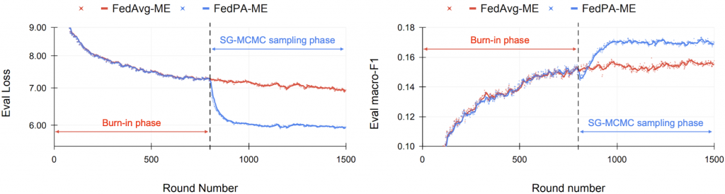
For clients to be able to sample from local posteriors using SG-MCMC, their models have to be close enough to local optima in the parameter space. Therefore, we first “burn-in” FedPA for a few rounds by running it in the FedAvg regime (i.e., compute the deltas the same way as FedAvg). At some point, we switch to local SG-MCMC sampling. Figures 4 and 5 show the evaluation metrics over the course of training. We clearly see a significant jump in performance right at the point when the algorithm was essentially switched from FedAvg to FedPA.
Concluding thoughts & what’s next?
Viewing federated learning through the lens of probabilistic inference turned out to be fruitful. Not only were we able to reinterpret FedAvg as a biased approximate inference algorithm and explain the strange effect of multiple local SGD steps on its convergence, but this new perspective allowed us to design a new FL algorithm that blends together optimization with local MCMC-based posterior sampling and utilizes local computation efficiently.
We believe that FedPA is just the beginning of a new class of approaches to federated learning. One of the biggest advantages of the distributed optimization over posterior inference so far is a strong theoretical understanding of FedAvg’s convergence and its variations in different IID and non-IID settings, which was developed over the past few years by the optimization community. Convergence analysis of posterior inference in different federated settings is an important research avenue to pursue next.
While FedPA relies on a number of specific design choices we had to make (the Laplace approximation, MCMC-based local inference, the shrinkage covariance estimation, etc.), our inferential perspective connects FL to a rich toolbox of techniques from Bayesian machine learning literature: variational inference, expectation propagation, ensembling and Bayesian deep learning, privacy guarantees for posterior sampling, among others. Exploring application of these techniques in different FL settings may lead us to even more interesting discoveries!
Want to learn more?
- Check out our ICLR 2021 paper.
- Play with all our FedPA demos using this code.
ACKNOWLEDGEMENTS: Thanks to Jenny Gillenwater, Misha Khodak, Peter Kairouz, and Afshin Rostamizadeh for feedback on this blog post.
DISCLAIMER: All opinions expressed in this post are those of the author and do not represent the views of CMU.
This article was initially published on the ML@CMU blog and appears here with the authors’ permission.

AUAI is supported by: