What is my data worth?

By Ruoxi Jia

People give massive amounts of their personal data to companies every day and these data are used to generate tremendous business values. Some economists and politicians argue that people should be paid for their contributions—but the million-dollar question is: by how much?

This article discusses methods proposed in our recent AISTATS and VLDB papers that attempt to answer this question in the machine learning context. This is joint work with David Dao, Boxin Wang, Frances Ann Hubis, Nezihe Merve Gurel, Nick Hynes, Bo Li, Ce Zhang, Costas J. Spanos, and Dawn Song, as well as a collaborative effort between UC Berkeley, ETH Zurich, and UIUC. More information about the work in our group can be found here.

What are the existing approaches to data valuation?

Various ad-hoc data valuation schemes have been studied in the literature and some of them have been deployed in the existing data marketplaces. From a practitioner’s point of view, they can be grouped into three categories:

• Query-based pricing attaches values to user-initiated queries. One simple example is to set the price based on the number of queries allowed during a time window. Other more sophisticated examples attempt to adjust the price to some specific criteria, such as arbitrage avoidance.
• Data attribute-based pricing constructs a price model that takes into account various parameters, such as data age, credibility, potential benefits, etc. The model is trained to match market prices released in public registries.
• Auction-based pricing designs auctions that dynamically set the price based on bids offered by buyers and sellers.

However, existing data valuation schemes do not take into account the following important desiderata:

• Task-specificness: The value of data depends on the task it helps to fulfill. For instance, if Alice’s medical record indicates that she has disease A, then her data will be more useful to predict disease A as opposed to other diseases.
• Fairness: The quality of data from different sources varies dramatically. In the worst-case scenario, adversarial data sources may even degrade model performance via data poisoning attacks. Hence, the data value should reflect the efficacy of data by assigning high values to data which can notably improve the model’s performance.
• Efficiency: Practical machine learning tasks may involve thousands or billions of data contributors; thus, data valuation techniques should be capable of scaling up.

With the desiderata above, we now discuss a principled notion of data value and computationally efficient algorithms for data valuation.

What would be a good notion for data value?

Due to the task-specific nature of data value, it should depend on the utility of the machine learning model trained on the data. Suppose the machine learning model generates a specific amount of profit. Then, we can reduce the data valuation problem to a profit allocation problem, which splits the total utility of the machine learning model between different data sources. Indeed, it is a well-studied problem in cooperative game theory to fairly allocate profits created by collective efforts. The most prominent profit allocation scheme is the Shapley value. The Shapley value attaches a real-value number to each player in the game to indicate the relative importance of their contributions. Specifically, for players, the Shapley value of the player () is defined as

where is the utility function that evaluates the worth of the player subset S. In the definition above, the difference in the bracket measures how much the payoff increases when player is added to a particular subset ; thus, the Shapley value measures the average contribution of player to every possible group of other players in the game.

Relating these game theoretic concepts to the problem of data valuation, one can think of the players as training data sources, and accordingly, the utility function as a performance measure of the model trained on the subset S of training data. Thus, the Shapley value can be used to determine the value of each data source. The Shapley value is appealing because it is the only profit allocation scheme that satisfies the following properties:

• Group rationality: the total utility of the machine learning model is completely split between different data sources, i.e., . This is a natural requirement because data contributors would expect the total benefit to be fully distributed.
• Fairness: Two data sources that have identical contributions to the model utility should have the same value; moreover, data sources with zero contributions to all subsets of the dataset should not receive any payoff.
• Additivity: The values under multiple utilities add up to the value under a utility that is the sum of all these utilities. This property generalizes the data valuation for a single task to multiple tasks. Specifically, if each task is associated with a utility function as the performance measure, with the additivity property, we can calculate the multi-task data value by simply computing the Shapley value with respect to the aggregated utility function.

Because the Shapley value uniquely satisfies the aforementioned properties and naturally leads to a payoff scheme dependent on the underlying task, we employ the Shapley value as a data value notion. While the outlined concept appears plausible, it has some fundamental challenges: computing the Shapley value, in general, requires evaluating the utility function for an exponential number of times; even worse, evaluating the utility function means re-training the model in the machine learning context. This is clearly intractable even for a small dataset. Interestingly, by focusing on the machine learning context, some opportunities arise to address the scalability challenge. Next, we show that for the K-nearest neighbors (KNN) classification, one can obviate the need to re-train models and compute the Shapley value in quasi-linear time—an exponential improvement in computational efficiency!

Efficient algorithms for KNN

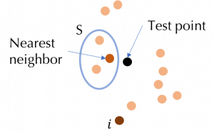
To understand why KNN is amenable to efficient data valuation, we consider and investigate the following simple utility function defined for 1NN: if the label of a test point is correctly predicted by its nearest neighbor in and otherwise. For a given test point, the utility of a set is completely determined by the nearest neighbor in this set to the test point. Thus, the contribution of the point to a subset is zero if the nearest neighbor in S is closer to the test point than . When we re-examine the Shapley value, we observe that for many , . Figure 1 illustrates an example of such an . This simple example shows the computational requirement of the Shapley value can be significantly reduced for KNN.

Figure 1: Illustration of why KNN is amenable to efficient Shapley value computation.

For a given test point , we let denote the th nearest neighbor in to the test point. Consider the following utility function that measures the likelihood of predicting the right label of a particular test point for KNN:

Now assume that the training data is sorted according to their similarity to the test point. We develop a simple recursive algorithm to compute the Shapley value of all training points from the furthest neighbor of the test point to the nearest one. Let represent the indicator function. Then, the algorithm proceeds as follows:

This algorithm can be extended to the case where the utility is defined as the likelihood of predicting the right labels for multiple test points. With the additivity property, the Shapley value for multiple test points is the sum of the Shapley value for every test point. The computational complexity is for training points and test points—this is simply the complexity of a sorting algorithm!

We can also develop a similar recursive algorithm to compute the Shapley value for KNN regression. Moreover, in some applications, such as document retrieval, test points could arrive sequentially and the value of each training point needs to be updated and accumulated on the fly, which makes it impossible to complete sorting offline. However, sorting a large dataset with a high dimension in an online manner will be expensive. To address the scalability challenge in the online setting, we develop an approximation algorithm to compute the Shapley value for KNN with improved efficiency. The efficiency boost is achieved by utilizing the locality-sensitive hashing to circumvent the need of sorting. More details of these extensions can be found in our paper.

Improving the efficiency for other ML models

The Shapley value for KNN is efficient due to the special locality structure of KNN. For general machine learning models, the exact computation of the Shapley value is inevitably slower. To address this challenge, prior work often resorts to Monte Carlo-based approximation algorithms. The central idea behind these approximation algorithms is to treat the Shapley value of a training point as its expected contribution to a random subset and use the sample average to approximate the expectation. By the definition of the Shapley value, the random set has size to with equal probability (corresponding to the factor) and is also equally likely to be any subset of a given size (corresponding to the factor). In practice, one can implement an equivalent sampler by drawing a random permutation of the training set. Then, the approximation algorithm proceeds by computing the marginal utility of a point to the points preceding it and averaging the marginal utilities across different permutations. This was the state-of-the-art method to estimate the Shapley value for general utility functions (referred to as the baseline approximation later). To assess the performance of an approximation algorithm, we can look at the number of utility evaluations needed to achieve some guarantees of the approximation error. Using Hoeffding’s bound, it can be proved that the baseline approximation algorithm above needs utility evaluations so that the squared error between the estimated and the ground truth Shapley value is bounded with high probability. Can we reduce the number of utility evaluations while maintaining the same approximation error guarantee?

We developed an approximation algorithm that requires only utility evaluations by utilizing the information sharing between different random samples. The key idea is that if a data point has a high value, it tends to boost the utility of all subsets containing it. This inspires us to draw some random subsets and record the presence of each training point in these randomly selected subsets. Denoting the appearance of the th and th training data by and . We can smartly design the distribution of the random subsets so that the expectation of is equal to . We can pick an anchor point, say, , and use the sample average of for all to estimate the Shapley value difference from all other training points to . Then, we can simply perform a few more utility evaluations to estimate , which allows us to recover the Shapley value of all other points. More details of this algorithm can be found in our paper. Since this algorithm computes the Shapley value by simply examining the utility of groups of data, we will refer to this algorithm as the group testing-based approximation hereinafter. Our paper also discusses even more efficient ways to estimate the Shapley value when new assumptions can be made, such as the sparsity of the Shapley values and the stability of the underlying learning algorithm.

Experiments

First, we demonstrate the efficiency of the proposed method to compute the exact Shapley value for KNN. We benchmark the runtime using a 2.6 GHZ Intel Core i7 CPU and compare the exact algorithm with the baseline Monte-Carlo approximation. Figure 2(a) shows the Monte-Carlo estimate of the Shapley value for each training point converges to the result of the exact algorithm with enough simulations, thus indicating the correctness of our exact algorithm. More importantly, the exact algorithm is several orders of magnitude faster than the baseline approximation as shown in Figure 2(b) .

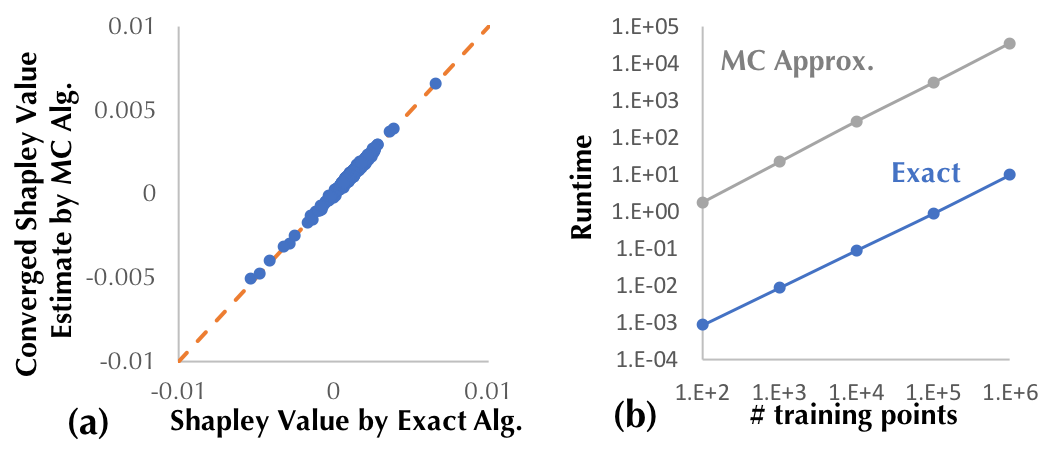Figure 2: (a) The Shapley value produced by our proposed exact approach and the baseline Monte-Carlo approximation algorithm for the KNN classifier constructed with 1000 randomly selected training points from MNIST. (b) Runtime comparison of the two approaches as the training size increases.

With the proposed algorithm, for the first time, we can compute data values for a practically large database. Figure 3 illustrates the result of a large-scale experiment using the KNN Shapley value. We take 1.5 million images with pre-calculated features and labels from Yahoo Flickr Creative Commons 100 Million (YFCC100m) dataset. We observe that the KNN Shapley value is intuitive—the top-valued images are semantically correlated with the corresponding test image. This experiment takes only a few seconds per test image on a single CPU and can be parallelized for a large test set.

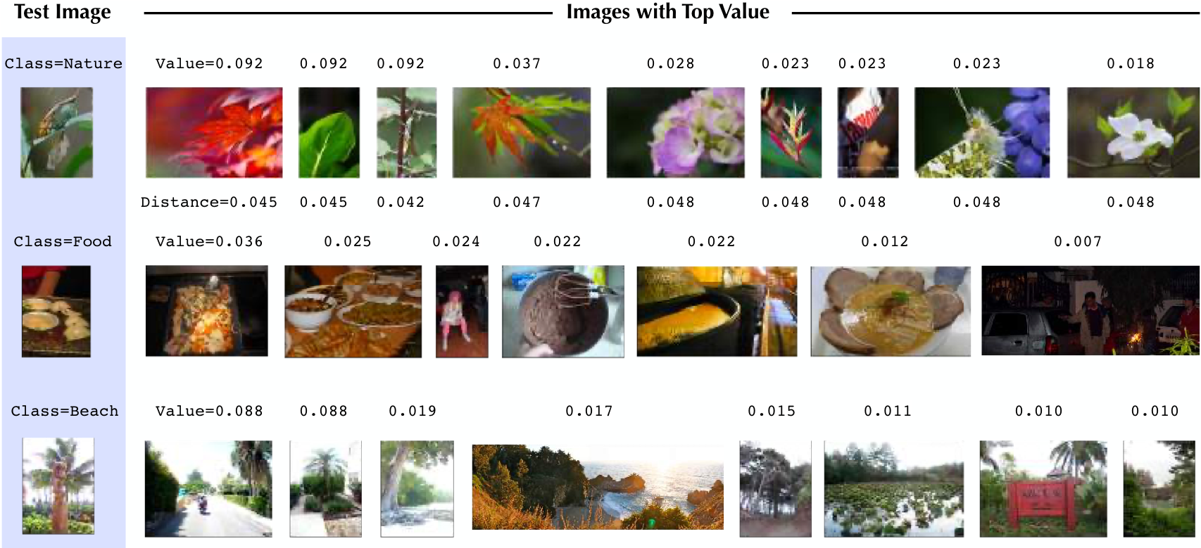Figure 3: Data valuation using KNN classifiers (K = 10) on 1.5 million images (all images with pre-calculated deep feature representations in the Yahoo100M dataset).

Similarly, Figure 4(a) demonstrates the accuracy of our proposed group testing-based approximation and Figure 4(b) shows that the group testing-based approximation outperforms the baseline approximation by several orders of magnitude for a large number of data points.

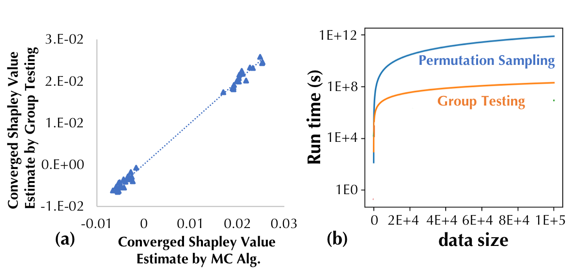Figure 4: The Shapley value produced by our proposed group testing-based approximation and the baseline approximation algorithm for a logistic regression classifier trained on the Iris dataset. (b) Runtime comparison of the two approaches.

We also perform experiments to demonstrate the utility of the Shapley value beyond data marketplace applications. Since the Shapley value tells us how useful a data point is for a machine learning task, we can use it to identify the low-quality or even adversarial data points in the training set. As a simple example, we artificially create a training set with half of the data directly from MNIST and the other half perturbed with random noise. In Figure 5, we compare the Shapley value between normal and noisy data as the noise ratio becomes higher. The figure shows that the Shapley value can be used to effectively detect noisy training data.

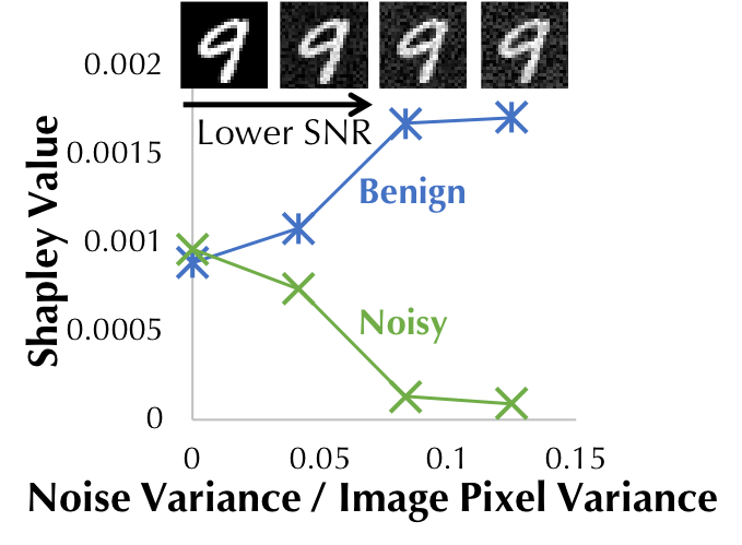
Figure 5: The Shapley value of normal and noisy training data as the noise magnitude becomes higher.

The Shapley value can also be used to understand adversarial training, which is an effective method to improve the adversarial robustness of a model by introducing adversarial examples to the training dataset. In practice, we measure the robustness in terms of the test accuracy on a dataset containing adversarial examples. We expect that the adversarial examples in the training dataset become more valuable as more adversarial examples are added into the test dataset. Based on the MNIST, we construct a training dataset that contains both benign and adversarial examples and synthesize test datasets with different adversarial-benign mixing ratios. Two popular attack algorithms, namely, the fast gradient sign method (FGSM) and the iterative attack (CW) are used to generate adversarial examples. Figure 6(a) and (b) compare the average Shapley value for adversarial examples and for benign examples in the training dataset. The negative test loss for logistic regression is used as the utility function. We see that the Shapley value of adversarial examples increases as the test data becomes more adversarial; in contrast, the Shapley value of benign examples decreases. In addition, the adversarial examples in the training set are more valuable if they are generated from the same attack algorithm during test time.

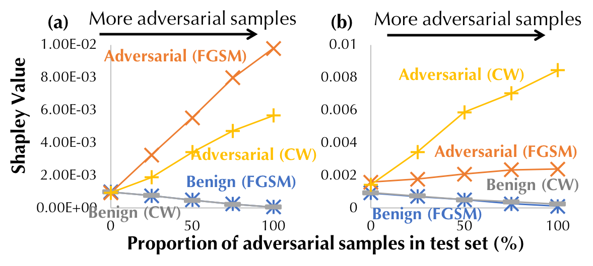Figure 6: Comparison of the Shapley value of benign and adversarial examples. FGSM and CW are different attack algorithms used for generating adversarial examples in the test dataset: (a) (resp. (b)) is trained on Benign+FGSM (resp. CW) adversarial examples.

Conclusion

We hope that our approaches for data valuation provide the theoretical and computational tools to facilitate data collection and dissemination in future data marketplaces. Beyond data markets, the Shapley value is a versatile tool for machine learning practitioners; for instance, it can be used for selecting features or interpreting black-box model predictions. Our algorithms can also be applied to mitigate the computational challenges in these important applications.

This article was initially published on the BAIR blog, and appears here with the authors’ permission.

BAIR blog

BAIR blog