
ΑΙhub.org
Learning DAGs with continuous optimization
By Xun Zheng, Bryon Aragam and Chen Dan
As datasets continually increase in size and complexity, our ability to uncover meaningful insights from unstructured and unlabeled data is crucial. At the same time, a premium has been placed on delivering simple, human-interpretable, and trustworthy inferential models of data. One promising class of such models are graphical models, which have been used to extract relational information from massive datasets arising from a wide variety of domains including biology, medicine, business, and finance, just to name a few.
Graphical models are families of multivariate distributions with compact representations expressed as graphs. In both undirected (Markov networks) and directed (Bayesian networks) graphical models, the graph structure guides the factorization of the joint distribution into smaller local specifications such as clique potentials  or local conditionals
  of a variable given its “parent” variables. At the same time, the graph structure also encodes the conditional independence relations among the variables.
Obviously, the graph structure is one of the crucial elements in defining graphical models. Often times, the structure of the graph reflects the human knowledge that guides the design of the graphical models: for instance, expert systems like the ALARM network use medical expertise to design a directed graphical model; the first-order Markov assumption on latent state dynamics leads to hidden Markov models; and deep belief networks believe that latent variables form a layer-wise structure. In these examples, the knowledge leads to the structure.
On the other hand, the structure can lead to the knowledge as well, especially in the scientific settings. For instance, estimating gene regulatory networks from gene expression data is an important biological inference task. Similarly, discovering the brain connectivity from brain imaging data can contribute immensely to our understanding of the brain. Even outside science, for instance in finance, being able to understand how different stocks influence each other can be important in making predictions.
The problem of estimating graphical model structure from the data is called structure learning. In this post, we will consider the structure learning of Bayesian networks, a problem closely related to other areas such as causality and interpretability.
Where are we?
| Markov networks (e.g., inverse covariance estimation) |
Bayesian networks (e.g., causal discovery) |
|
| Constraint-based | Dempster (1972) | Spirtes, Glymour (1991) |
| Score-based (local search, combinatorial) |
Pietra et al. (1997) | Heckerman et al. (1995) |
| Score-based (global search, continuous) |
Meinshausen, Bühlmann (2006) Yuan, Lin (2007) Banerjee et al. (2008) Friedman et al. (2008) Ravikumar et al. (2010, 2011) … |
? |
The history of structure learning in Markov networks and Bayesian networks share a similar pattern: from constraint-based to score-based, and from local search to global search.
Constraint-based methods try to test conditional independencies from the data  , and uses them to construct a compatible graphical model
  :
:
![\[X \xrightarrow{\textit{hypothesis test}} \textit{independence set} \xrightarrow{\textit{I-map}} G\]](https://aihub.org/wp-content/ql-cache/quicklatex.com-d3560acd83a5c0c94cf3983de1268d07_l3.png "Rendered by QuickLaTeX.com")
There are several limitations to this approach: the first step is sensitive to individual failures of tests; the second step requires faithfulness, which is a strong assumption.
Score-based methods define an  -estimator for some score function that measures how well the graph fits the data:
![\[\max_G \ \mathit{score}(G; X)\]](https://aihub.org/wp-content/ql-cache/quicklatex.com-42465e51fc6389083baf6eceec613916_l3.png "Rendered by QuickLaTeX.com")
Because of the large search space, the problem is in general NP-hard. Moreover, since this is a combinatorial problem, it often resorts to local search heuristics, which in turn makes implementation particularly difficult.
In the 2000s, we witnessed a significant breakthrough in the structure learning problem for Markov networks. Instead of using a local search, which optimizes one edge at a time, these methods recast the optimization problem as a continuous program and perform a global search: They search and update the entire graph in each iteration. This was made possible by treating the score-based learning problem as a continuous optimization program. This led to the huge success of methods like graphical lasso in practical fields like bioinformatics.
A natural question is then:
Can we use continuous optimization to perform a global search in score-based learning for Bayesian networks?
The main difficulty is that unlike the graphical lasso, which is a convex continuous program, Bayesian networks lead to a nonconvex combinatorial program: the graph has to be acyclic. How can we incorporate this constraint into the continuous optimization problem?
A smooth characterization of acyclicity
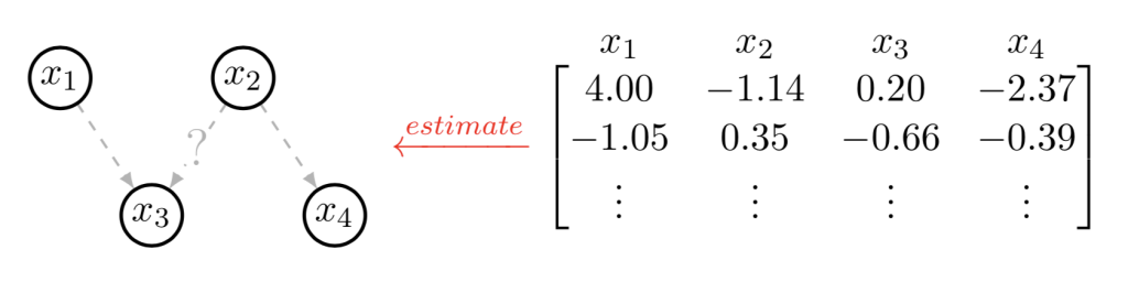
Let’s first focus on the case of linear DAGs, where each child variable depends linearly on its parents. In this case, the zero element of the weighted adjacency matrix  naturally represents the absence of the corresponding edge in the graph . Our goal is to estimate a , or equivalently a , that fits the data best.
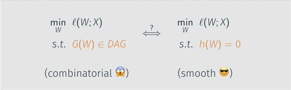
![\[\begin{aligned} \min_G & \ \ell(G; X) \\ \mathit{s.t.}\ & \ {G \in \textit{DAG}}\end{aligned}\quad \iff \quad\begin{aligned}\min_W & \ \ell(W; X) \\\mathit{s.t.} \ & \ {h(W) = 0}\end{aligned}\]](https://aihub.org/wp-content/ql-cache/quicklatex.com-43664b19990a7240c8713e05ef08a6cc_l3.png "Rendered by QuickLaTeX.com")
Essentially, we would like to transform the traditional combinatorial problem for graph (left) into a continuous optimization program over weighted adjacency matrices (right). The key technical device is the smooth function  whose level set at zero is equivalent to the set of DAGs.
In our paper, we showed that such a function  exists,
![\[{h(W)} = \mathrm{tr} (e^{W \circ W}) - d,\]](https://aihub.org/wp-content/ql-cache/quicklatex.com-fba9ca50958e6636e02995f11f7e4c47_l3.png "Rendered by QuickLaTeX.com")
and that it has a simple gradient:
![\[\nabla h(W) = (e^{W \circ W})^T \circ 2W.\]](https://aihub.org/wp-content/ql-cache/quicklatex.com-046f3395f37b8b4d25da5eb7b928c79a_l3.png "Rendered by QuickLaTeX.com")
Here the  is the element-wise product,
  is the size of the graph,
  is the trace of a matrix, and the matrix exponential is defined as the infinite power series
![\[e^A = I + A + \frac{1}{2!} A^2 + \frac{1}{3!} A^3 + \cdots\]](https://aihub.org/wp-content/ql-cache/quicklatex.com-72dfb3e8d3daa843e356a74c37a81306_l3.png "Rendered by QuickLaTeX.com")
The intuition behind this function is that the  -th power of the adjacency matrix of a graph counts the number of -step paths from one node to another. In other words, if the diagonal of the matrix power turns out to be all zeros, there is no -step cycles in the graph. Then to characterize acyclicity, we just need to set this constraint for all
  , eliminating cycles of all possible length.
Equipped with this smooth characterization of DAGs , now the new -estimator reduces to a continuous optimization problem with a nonlinear equality constraint. This is interesting for several reasons:
- The hard work of edge search can now be delegated to numerical solvers, instead of being implemented by experts in graphical models.
- From an optimization point of view, this approach is agnostic to properties of the graph, whereas traditional methods typically require assumptions such as bounded degree or tree-width.
- Similar to sparse inverse covariance estimation for high-dimensional Gaussian graphical model selection, it is straightforward to incorporate structural regularization such as sparsity.
NO TEARS
TEARS
Now that we have an M-estimator entirely written as a continuous constrained optimization program (albeit nonconvex), standard numerical algorithms such as augmented Lagrangian can be employed. At a high level, this involves two steps:
- Minimize augmented primal (continuous, unconstrained):

- Dual ascent (1-dimensional update):

The entire algorithm can be written in less than 50 lines of Python: 30 lines for the function/gradient definitions, and 20 lines for the augmented Lagrangian as shown above. For interested readers, the complete algorithm with executable example is publicly available on Github. To highlight the simplicity, we decided to name it NOTEARS: Non-combinatorial Optimization via Trace Exponential and Augmented lagRangian for Structure learning.
Recovering random graph structures
Below, we visualize the iterates of the aforementioned augmented Lagrangian scheme. Since the parameter here is simply a weighted adjacency matrix, we can visualize this with a heatmap. On the left is the ground truth, the middle is an animation showing each iterate, and on the right is the difference between the current iterate and the ground truth.
We can validate the algorithm by simulating random graphs as the ground truth, for instance an Erdős–Rényi graph, where edges take place independently with certain probability. It is clear that the NOTEARS algorithm quickly recovers the true DAG structure, as well as the edge weights.
Earlier we claimed that one advantage of the optimization view is that the algorithm is agnostic about graph properties. Indeed, the next example illustrates an example in which the degree distribution of the ground truth is highly unbalanced, and for which our algorithm can still recover the graph efficiently. This example is generated from a scale-free graph, where some nodes are much more heavily connected than the rest.
Moving forward: from linear to nonlinear
So far we have assumed linear dependence between random variables – i.e., we are working with linear structural equation models (SEM):
![\[X_j = \sum_{i \in \mathrm{pa}(j)} W_{ij} X_i + Z_j\]](https://aihub.org/wp-content/ql-cache/quicklatex.com-18a9aaed90fca896edf60b26d347f697_l3.png "Rendered by QuickLaTeX.com")
where  is the independent noise with zero mean. It can be naturally extended to account for certain nonlinear transformations in the same way generalized linear models (GLMs) extend linear regression:
![\[\mathbb{E} \left[X_j | X_{\mathrm{pa}(j)} \right] = g_j \left(\sum_{i \in \mathrm{pa}(j)} W_{ij} X_i \right)\]](https://aihub.org/wp-content/ql-cache/quicklatex.com-07be95c445c87748e50bf1202a7ec1d2_l3.png "Rendered by QuickLaTeX.com")
with mean function  . However, a fully nonlinear model in terms of
  still remains nontrivial. The question is then:
Can we use continuous optimization to learn nonparametric DAGs?
The model of consideration is now generalized to nonparametric SEMs:
![\[\mathbb{E} \left[X_j | X_{\mathrm{pa}(j)} \right] = g_j \left(f_j(X)\right),\]](https://aihub.org/wp-content/ql-cache/quicklatex.com-ce6bedcc59ded4772240a0e2414361c2_l3.png "Rendered by QuickLaTeX.com")
where the (possibly nonlinear) function  does not depend on
  if
if  in .
in .
Notice that in linear SEMs the weighted adjacency matrix plays two different roles: is the parameterization of the SEM, but at the same time, it also induces the graph structure. This is an important fact that enables the continuous optimization strategy in NOTEARS.
Once we move to the nonparametric SEM, however, there is no such in the first place! How can we “smoothly” connect the score function and the acyclicity constraint?
A notion of nonparametric acyclicity
Luckily, partial derivatives can be used to measure the dependence of  on the -th variable, an idea that dates back to at least Rosasco et al. Essentially, is independent of
  if and only if
  . Then we can construct the following matrix that encodes the dependency structure between variables:
![\[W(f) = W(f_1, \dotsc, f_d) \in \mathbb{R}^{d \times d}, \quad [W(f)]_{kj} := \| \partial_k f_j \|_{L^2}.\]](https://aihub.org/wp-content/ql-cache/quicklatex.com-190e8f735dc1f966fdfad95c952a7a0f_l3.png "Rendered by QuickLaTeX.com")
The resulting continuous M-estimator is then:
![\[\min_{f=(f_1, \dotsc, f_d)} \ell(f; X) \quad \text{s.t.} \quad h(W(f)) = 0.\]](https://aihub.org/wp-content/ql-cache/quicklatex.com-b5c57cc4c6d25c16c5a6efa358ba452f_l3.png "Rendered by QuickLaTeX.com")
One can immediately notice that when are linear, this reduces to the linear NOTEARS. Moreover, in our recent paper, we show that it subsumes a variety of parametric and semiparametric models including additive noise models, generalized linear models, additive models, and index models.
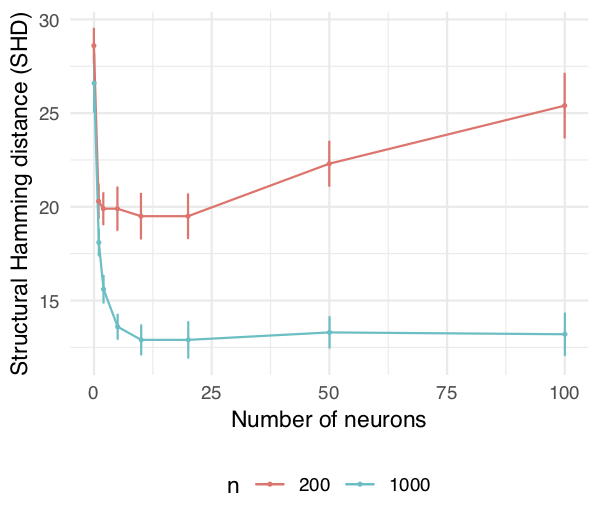
The remaining question is: How do we actually solve it? In general, the above program is infinite-dimensional, so we choose a suitable family of approximations (e.g. neural networks, orthogonal series, etc.) to reduce this to a tractable optimization problem over a finite-dimensional parameter  . Notably, for both multi-layer perceptrons and Sobolev basis expansions,
  is smooth w.r.t. . Hence we again arrive at a problem ready for off-the-shelf numerical solvers. In particular, even a relatively simple neural network like 1-hidden-layer multi-layer perceptron with 10 hidden units suffices to capture nonlinear relationships between variables.
Concluding remarks
Score-based global search of Bayesian networks using continuous optimization has thus far been missing from the existing literature. We hope our work serves as a first step toward filling this gap between undirected and directed graphical model selection. The key technical device is the notion of acyclicity that leverages SEM parameters in the algebraic characterization of DAGs.
Since the algebraic characterization of DAG is exact, it inherits the nonconvexity of DAG learning. Nonetheless, the stationary point is often good enough. An interesting future direction is to study the nonconvex landscape of the continuous M-estimator more carefully in order to provide rigorous guarantees on the optimality of the solutions.
For more details, please refer to the following resources:
- X. Zheng, B. Aragam, P. Ravikumar, E. P. Xing. DAGs with NO TEARS: Continuous Optimization for Structure Learning. Advances in Neural Information Processing Systems (NeurIPS), 2018.
- X. Zheng, C. Dan, B. Aragam, P. Ravikumar, E. P. Xing. Learning Sparse Nonparametric DAGs. International Conference on Artificial Intelligence and Statistics (AISTATS), 2020.
DISCLAIMER: All opinions expressed in this post are those of the author and do not represent the views of CMU.
This article was initially published on the ML@CMU blog and appears here with the authors’ permission.

AUAI is supported by: