Simultaneous clustering and representation learning

The success of deep learning over the last decade, particularly in computer vision, has depended greatly on large training data sets. Even though progress in this area boosted the performance of many tasks such as object detection, recognition, and segmentation, the main bottleneck for future improvement is more labeled data. Self-supervised learning is among the best alternatives for learning useful representations from the data. In this article, we will briefly review the self-supervised learning methods in the literature and discuss the findings of a recent self-supervised learning paper from ICLR 2020 [14].

What is self-supervised learning?

We may assume that most learning problems can be tackled by having clean labeling and more data obtained in an unsupervised way. However, acquiring labeled data in many tasks requires laborious manual annotation and expert knowledge. Sometimes, even though there are more convenient methods for labeling label data, such as crowdsourcing, it may not be an option when working with private data. Additionally, human-curated datasets are only a minuscule of data produced every day. Self-supervised learning aims to learn meaningful representations from unlabelled data and eventually transfer those learned representations to primary tasks.

Self-supervised learning is done by learning an auxiliary (surrogate) task that can be obtained from unlabeled data and help in one or more tasks. Depending on the tasks, these auxiliary tasks aim to learn spatial, contextual, or temporal relations on different modalities. Focusing on computer vision tasks, we can give several examples of auxiliary tasks: image colorization [15], predicting the relative spatial configurations of two given image patches [6], ordering image patches shuffled like jigsaw puzzles [10], learning to predict the rotation of a given image [7], learning to generate future frames in videos [11], learning to predict whether video frames are in a temporally correct or incorrect order [9], predicting whether a video is playing forward or backward (arrow of time) [12].

In addition to these auxiliary tasks, there is self-supervised learning in different modalities such as audio and text. Furthermore, it is even possible to apply self-supervision to multimodal data (i.e. vision, audio, and language) [2,1,8].

Representation learning by clustering

First, we review DeepCluster and then discuss the motivation and the main contribution of the self-labeling paper by Yuki Asano, Christian Rupprecht and Andrea Vedaldi [14]. Figure 1 shows the general idea of deep clustering. The output of a convolutional neural network is used as a feature representation; k-means clustering is applied on top of this. The representation is improved by learning those cluster IDs as labels using a cross-entropy loss. One question concerns the initial representation. A multilayer perceptron using randomly initialized AlexNet’s last convolutional layer as feature representation performs 12% on ImageNet, whereas the change level is 0.1%. Considering there are 1000 categories in ImageNet, 12% top-1 accuracy using a random network’s features and a simple MLP classifier can be regarded as good because the network is not trained on any labeled data. Thus, convolutional networks have a strong prior on the input data and can be used to initialize clustering-based representation learning.

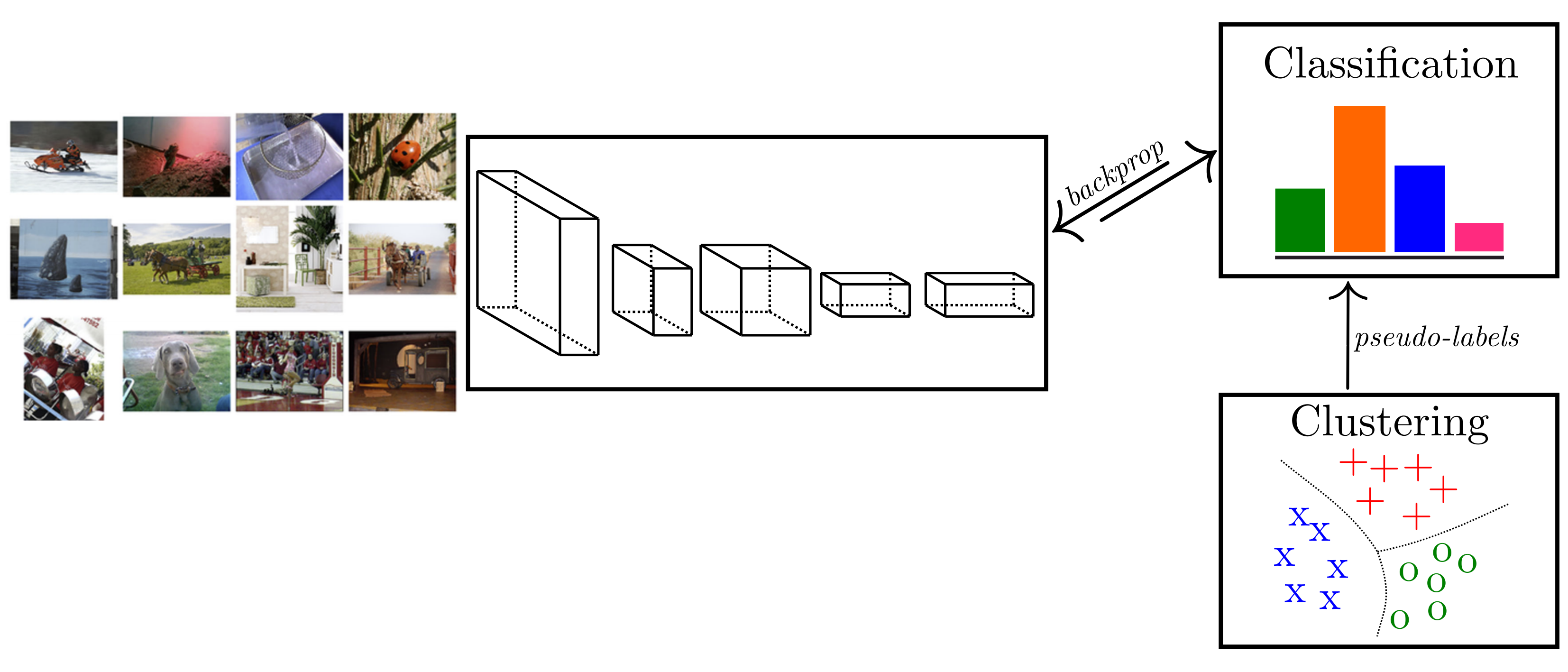
The main problem of k-means or other clustering methods (in DeepCluster) is degeneracy. This means that one or more cluster centers are empty (no entities assigned to them), or two or more cluster centers are identical. Furthermore, the imbalanced distribution of training samples may lead to accumulation of the majority of samples in a few clusters, affecting the network’s parameterization. In the worst-case scenario, the network predicts the same output for all. The solution in [3] for an empty cluster during optimization is to randomly select a non-empty cluster and use its centroid by small perturbation as a new cluster. For the imbalanced training data, the authors proposed uniform sampling over the pseudo-labels.

Self-labeling via simultaneous clustering and representation learning

Asano et al. [14] proposed a method to perform clustering and representation learning under the same objective simultaneously. To prevent degenerate solutions, they assumed the number of training samples from each class should be similar, and induced the equipartition constraint by addressing the self-labeling as an optimal transport problem. To scale up large datasets with millions of data points, they approximated the transport problem using the Sinkhorn-Knopp algorithm.

Let’s have a closer look at the self-labeling (SeLa) approach. A deep neural network maps the input images to feature vectors . In a supervised setting, the model is trained with N data points and labels . The classification is done by a single fully connected layer on top of feature vectors. The parameters are learned by minimizing the average cross-entropy loss:

(1)  

The same approach may also work in a semi-supervised setting where only a part of the training samples are labelled. If the posterior distribution is set to be deterministic, the formulation above can be written as follows:

(2)  

When assigning labels, adding the constraint of equally-sized subsets can prevent degeneracy. The learning objective becomes

(3)  

Each label is assigned to data points uniformly, and each data point can take only one label. Together with these constraints, the objective becomes combinotarial in . This is an example of an optimal transport problem. Let be the matrix of joint probabilities estimated by the model, and the matrix of assigned joint probabilities. Matrix can be relaxed to be an element of the transportation polytope

(4)  

Here, all s are vectors of all ones, and and are the marginal projections of on its rows and columns. The uniform distribution constraint is fulfilled by . Then, the objective becomes

(5)  

Instead of eq. (3), by constant shift of , we can solve

(6)  

Now, this problem is called the optimal transport between and . It is a linear program and can be solved in polynomial time. In practice, traditional solvers scale badly – to the millions of instances. Thus, the authors adapted a fast approximate version of the Sinkhorn-Knopp algorithm (proposed in [5]):

(7)  

According to Sinkhorn’s theorem, matrix that holds the joint probabilities can be written as . Then, the problem turns into a matrix scaling iteration.

To summarize the algorithm, both the model and the label assignment matrix are learned by optimizing There are two alternating steps:
1) Updating the parameters of the model using the current label assignments (learning representation)
2) Given the current model, computing the log probabilities and finding by matrix scaling (self-labeling)

The self-labeling approach has a single matrix-vector multiplication and has a complexity of According to the paper, the convergence is reached in two minutes in ImageNet in more than million images and several thousands of clusters.

For more details about the optimal transport problem and Sinkhorn-Knopp algorithm, I recommend that interested readers check Cuturi et al. [5]. This blog post is also very informative and explains Sikhorn distances very well.

Experimental Results

In self-supervised representation papers, the standard evaluation for comparing the representative power of different features (typically using the same network, e.g., AlexNet) applies only a linear classifier on top of them. As training data, ImageNet LSVRC-12 and MIT Places were used.

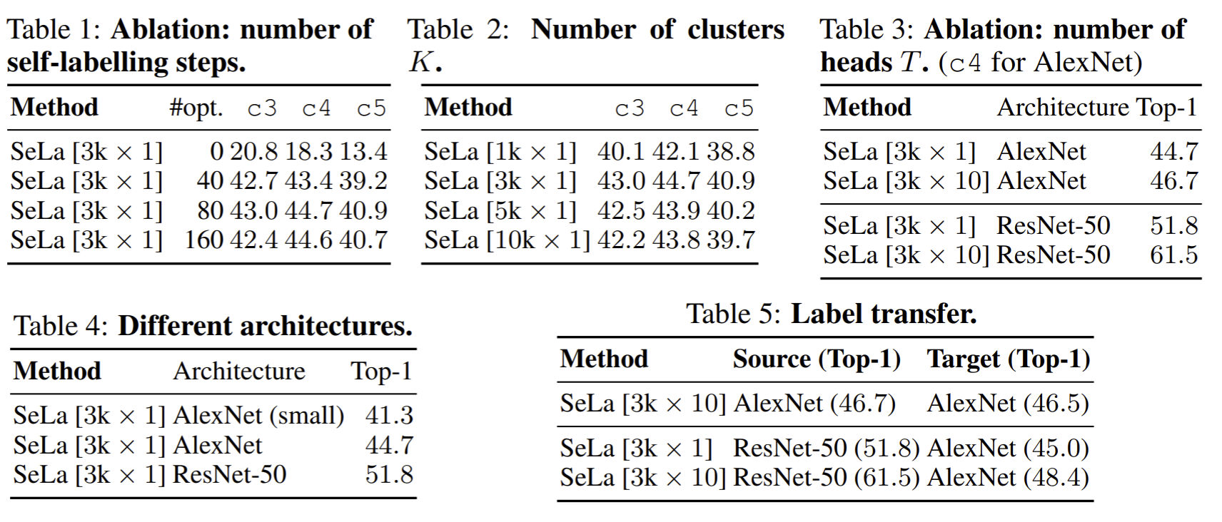
Rigorous ablation studies were carried out to find optimal configurations. Those results are given in Table 1. The design choices are

• the number of self-labeling steps,
• the number of clusters,
• the number of classification heads,
• network architecture,
• the label transfer performance.

Clustering can be performed on different tasks, and each can capture similarities based on shape, color, or geometry. The authors experimented with multiple classification heads on top of the same network (labels of each task were acquired by different self-labeling steps).

An impressive result is that the labels acquired by self-labeling are transferable. When the final self-labels are used to train either the same or different network architecture, for instance, labels acquired by ResNet-50 can help to train an AlexNet that performs better when trained itself using self-labeling. The best configuration is achieved with 3k clusters, multi-task setting (10 classification heads), and ResNet-50 architecture after approx. 80 self-labeling steps.

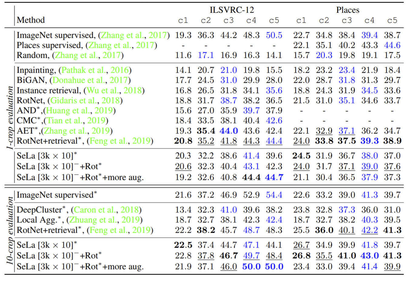
Comparison with other self-supervised methods In large-scale benchmarks, the most established benchmark is AlexNet and linear probing on ImageNet and MIT Places datasets. The self-labeling approach outperforms many self-supervised methods, including inpainting, BiGAN, rotation, and more recent approaches such as contrastive multiview coding, and autoencoding transformations.

When ResNet-50 architecture is used, SeLa performs better than most previous approaches (61.5% top-1 accuracy). In general, clustering-based representation learning methods require less tuning than other specialized pre-tasks. A recent work that is a current state-of-the-art, Swapping Assignments between multiple Views of the same image (SwAV) [4], enforces consistency between different augmentations (views) of the same image. Instead of comparing features, the authors predict the cluster assignment of a view from the representation of another view and reached 75.3% top-1 accuracy in ImageNet using ResNet-50. More interestingly, they used the equipartition constraint of [14] in an online setting in mini-batches.

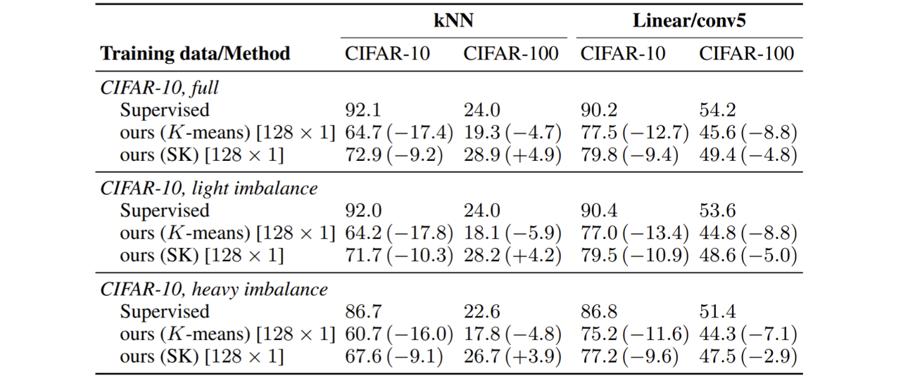
Training on imbalanced datasets

In practice, we cannot easily find balanced datasets in many problems; however, the ImageNet training set is equally distributed. Even though the motivation behind the Sinhkorn-Knopp (SK) algorithm and the self-labeling is to prevent clustering degeneracy, it may be an issue in imbalanced datasets. To address this question, the authors performed experiments in CIFAR-10 and CIFAR-100 by creating light and heavy imbalanced sets. SK performs better than k-means. It shows that their method can learn discriminative representations even when trained on imbalanced datasets.

Where to stop training auxiliary tasks (clustering)? In most self-supervised tasks, training heuristics are experimentally validated. Training more on the auxiliary tasks can cause overfitting and deteriorate the performance on object retrieval/classification tasks. In SeLa, the pseudo-labels are changed at intervals; thus, the problem keeps changing. The normalized mutual information (NMI) between the self-labels and ImageNet labels in the validation set (reported in the appendix) seems to increase very quickly and then remains fairly constant up to 400 epochs.

Finetuning on different tasks and dataset When the AlexNet trained with SeLa is finetuned on the PASCAL VOC benchmark, it outperforms the supervised baseline in detection tasks, and reaches comparable performance in classification and segmentation tasks. Finetuning the entire network gives better results than finetuning only the classification head (fc6-8). There is still a difference between the representation ability of Conv1-5 in self-supervised and supervised methods. To some extent, this seems natural as we expect learning low-level features are easier than mid- and high-level features. In another ICLR’20 paper from the same authors [13] they compared the Conv1-5 features trained on a single image with strong augmentation and full supervision. They conclude that low-level image statistics can be learned even from a single image (and strong data augmentation); however, there is a gap in higher convolutional layers even though millions of images were used. The performance gap between SeLa and the supervised baseline can be seen in Table 9 of the paper (i.e., 44.3/48.3, 44.4/50.5 in the layers of AlexNet conv4-5 on ImageNet 1-crop evaluation).

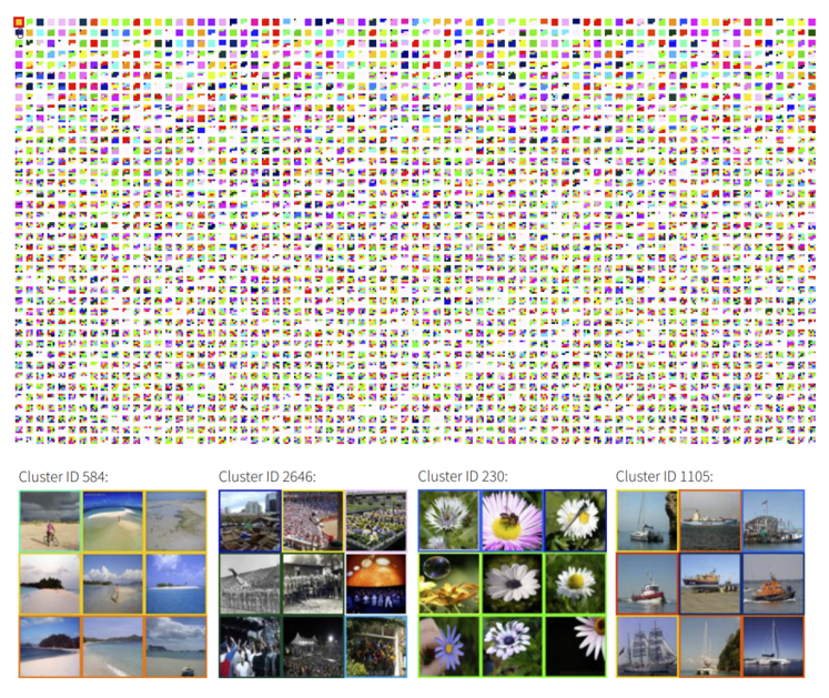
In their blog post, the authors of SeLa provided an online visualization tool that shows nine sampled images from all 3000 clusters trained using their method. Even though those images per cluster do not belong to the same category, it is clear that they look visually similar (in terms of context, object type, and color, background).

Concluding Remarks

To sum up, we covered the details of a self-labeling approach that enforces equipartition constraints in clustering-based representation learning. The paper addressed this constraint as an optimal transport problem and used a fast version of the Sinkhorn-Knopp algorithm.

In contrast to other self-supervised methods (i.e., inpainting, patch context, and rotation) that are restricted to a specific domain, clustering-based approaches can be applied in different modalities (for instance, DeepCluster applied to video and audio domains). If you are interested in learning visual features by clustering, I recommend reading DeepCluster [3], this paper on self-labeling [14], and the more recent follow-up to both papers [4].

Note: All tables and figures taken from SeLa [14] are used with permission from the authors.

References

[1] Jean-Baptiste Alayrac, Adrià Recasens, Rosalia Schneider, Relja Arandjelović, Jason Ramapuram, Jeffrey De Fauw, Lucas Smaira, Sander Dieleman, and Andrew Zisserman. Self-supervised multimodal versatile networks (2020).
[2] Yusuf Aytar, Carl Vondrick, and Antonio Torralba. See, hear, and read: Deep aligned representations (2017).
[3] Mathilde Caron, Piotr Bojanowski, Armand Joulin, and Matthijs Douze. Deep clustering for unsupervised learning of visual features. (2018).
[4] Mathilde Caron, Ishan Misra, Julien Mairal, Priya Goyal, Piotr Bojanowski,and Armand Joulin. Unsupervised learning of visual features by contrasting cluster assignments (2020).
[5] Marco Cuturi. Sinkhorn distances: Lightspeed computation of optimal transport (2013).
[6] C. Doersch, A. Gupta, and A. A. Efros. Unsupervised visual representation learning by context prediction (2015).
[7] Spyros Gidaris, Praveer Singh, and Nikos Komodakis. Unsupervised representation learning by predicting image rotations (2018).
[8] David Harwath, Adrià Recasens, Dídac Surís, Galen Chuang, Antonio Torralba, and James Glass. Jointly discovering visual objects and spoken words from raw sensory input (2018).
[9] Ishan Misra, C. Lawrence Zitnick, and Martial Hebert. Shuffle and learn: Unsupervised learning using temporal order verification (2016).
[10] Mehdi Noroozi and Paolo Favaro. Unsupervised learning of visual representations by solving jigsaw puzzles (2016).
[11] Nitish Srivastava, Elman Mansimov, and Ruslan Salakhutdinov. Unsupervised learning of video representations using LSTMs (2015).
[12] Donglai Wei, Joseph J. Lim, Andrew Zisserman, and William T. Freeman. Learning and using the arrow of time (2018).
[13] Asano YM., Rupprecht C., and Vedaldi A. A critical analysis of self-supervision, or what we can learn from a single image (2020).
[14] Asano YM., Rupprecht C., and Vedaldi A. Self-labelling via simultaneous clustering and representation learning (2020).
[15] Richard Zhang, Phillip Isola, and Alexei A. Efros. Colorful image colorization. In Computer Vision – ECCV (2016). Also see webpage.

Ömer Sümer is a third-year PhD candidate in computer science and a research assistant at the University of Tübingen.

Ömer Sümer is a third-year PhD candidate in computer science and a research assistant at the University of Tübingen.