☰

ΑΙhub.org

Reinforcement learning is supervised learning on optimized data

by BAIR blog

05 November 2020

Common Perspectives on RL

In this section, we will describe the two predominant perspectives on RL.

Optimization Perspective

The optimization perspective views RL as a special case of optimizing non-differentiable functions. Recall that the expected reward is a function of the parameters $\theta$ of a policy $\pi_\theta$ :

$J(\theta) = \mathbb{E}_{s' \sim p(s' \mid s, a), a \sim \pi(a \mid s)} \left[\sum_t \gamma^t r(s_t, a_t) \right].$

This function is complex and usually non-differentiable and unknown, as it depends on both the actions chosen by the policy and the dynamics of the environment. While we can estimate the gradient using the REINFORCE trick, this gradient depends on the policy parameters and on-policy data, which is generated from the simulator by running the current policy.

Dynamic Programming Perspective

The dynamic programming perspective says that optimal control is a problem of choosing the right action at each step. In discrete settings with known dynamics, we can solve this dynamic programming problem exactly. For example, Q-learning estimates the state-action values, $Q(s, a)$ by iterating the following updates:

$Q(s, a) \gets r(s, a) + \gamma \max_{a'} \mathbb{E}_{s' \sim p(s' \mid s, a)}[Q(s', a')].$

In continuous spaces or settings with large state and action spaces, we can approximate dynamic programming by representing the Q-function using a function approximator (e.g., a neural network) and minimizing the difference the TD error, which is the squared-difference between the LHS and RHS in the equation above:

$TD(\theta) = \frac{1}{2}(Q_\theta(s, a) - y(s, a))^2,$

where the TD target $y(s, a) = r(s, a) + \gamma \max_{a'} Q_\theta(s', a')$ . Note that this is a loss function for the Q-function, instead of the policy.

This approach allows us to use any kind of data for optimizing the Q-function, therefore preventing the need to have “good” data, but it suffers from major optimization issues and can diverge or converge to poor solutions and can be hard to apply to new problems.

Supervised Learning Perspective

We now discuss another mental model for RL. The main idea is to view RL as a joint optimization problem over the policy and experience: we simultaneously want to find both “good data” and a “good policy.” Intuitively, we expect that “good” data will (1) get high reward, (2) sufficiently explore the environment, and (3) be at least somewhat representative of our policy. We define a good policy as simply a policy that is likely to produce good data.

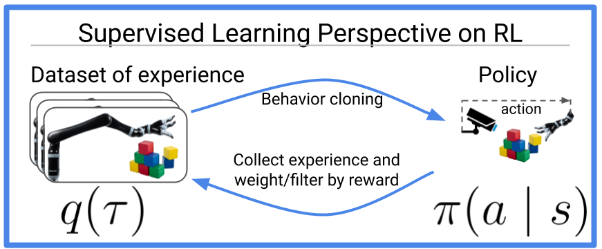
Figure 1: Many old and new reinforcement learning algorithms can be viewed as doing
behavior cloning (a.k.a. supervised learning) on optimized data. This blog post
discusses recent work that extends this idea to the multi-task perspective,
where it actually becomes *easier* to optimize data.

Converting “good data” into a “good policy” is easy: just do supervised learning! The reverse direction, converting a “good policy” into “good data” is slightly more challenging, and we’ll discuss a few approaches in the next section. It turns out that in the multi-task setting or by artificially modifying the problem definition slightly, converting a “good policy” into “good data” is substantially easier. The penultimate section will discuss how goal relabeling, a modified problem definition, and inverse RL extract “good data” in the multi-task setting.

An RL objective that decouples the policy from data

We now formalize the supervised learning perspective using the lens of expectation maximization, a lens used in many prior works [Dayan 1997, Williams 2007, Peters 2010, Neumann 2011, Levine 2013]. To simplify notation, we will use $\pi_\theta(\tau)$ as the probability that policy $\pi_\theta$ produces trajectory $\tau$ , and will use $q(\tau)$ to denote the data distribution that we will optimize. Consider the log of the expected reward objective, $\log J(\theta)$ . Since log function is monotonic increasing, maximizing this is equivalent to maximizing the expected reward. We then apply Jensen’s inequality to move the logarithm inside the expectation:

What’s useful about this lower bound is that it allows us to optimize a policy using data sampled from a different policy. This lower bound makes explicit the fact that RL is a joint optimization problem over the policy and experience. The table below compares the supervised learning perspective to the optimization and dynamic programming perspectives:

	Optimization Perspective	Dynamic Programming Perspective	Supervised Learning Perspective
What are we optimizing?	policy ( $\pi_\theta$ )	Q-function ( $Q_\theta$ )	policy ( $\pi_\theta$ ) and data ( $q(\tau)$ )
Loss	Surrogate loss $\tilde{L}(\theta, \tau \sim \pi_\theta)$	TD error	Lower bound $F(\theta, q)$
Data used in loss	collected from current policy	arbitrary	optimized data

Finding good data and a good policy correspond to optimizing the lower bound, $F(\theta, q)$ , with respect to the policy parameters and the experience. One common approach for maximizing the lower bound is to perform coordinate ascent on its arguments, alternating between optimizing the data distribution and the policy.¹

Optimizing the Policy

When optimizing the lower bound with respect to the policy, the objective is (up to a constant) exactly equivalent to supervised learning (a.k.a. behavior cloning)!

$\max_\theta F(\theta, q) = \max_\theta \mathbb{E}_{\tau \sim q(\tau)} \left[\sum_{s_t, a_t \in \tau} \log \pi_\theta(a_t \mid s_t) \right] + \text{const.}$

This observation is exciting because supervised learning is generally much more stable than RL algorithms². Moreover, this observation suggests that prior RL methods that use supervised learning as a subroutine[Oh 2018, Ding 2019] might actually be optimizing a lower bound on expected reward.

Optimizing the Data Distribution

The objective for the data distribution is to maximize reward while not deviating too far from the current policy.

$\max_q F(\theta, q) = \max_q \mathbb{E}_{q(\tau)} \left[ \log R(\tau) \right] - D_\text{KL}\left(q(\tau) \; \| \; \pi(\tau) \right).$

The KL constraint above makes the optimization of the data distribution conservative, preferring to stay close to the current policy at the cost of slightly lower reward. Optimizing the expected log reward, rather than the expected reward, further makes this optimization problem risk averse (the $\log(\cdot)$ function is a concave utility function[^Ingersoll19]).

There are a number of ways we might optimize the data distribution. One straightforward (if inefficient) strategy is to collect experience with a noisy version of the current policy, and keep the 10% of experience that receives the highest reward.[^Oh18] An alternative is to do trajectory optimization, optimizing the states along a single trajectory.[Neumann 2011, Levine 2013] A third approach is to not collect more data, but rather reweight previous collected trajectories by their reward. [Dayan1997] Moreover, the data distribution $q(\tau)$ can be represented in multiple ways – as a non-parametric discrete distribution over previously-observed trajectories[Oh 2018], or a factored distribution over individual state-action pairs [Neumann 2011, Levine 2013] or as a semi-parametric model that extends observed experience with extra hallucinated experience generated from a parametric model.[Kumar 2019]

Viewing Prior Work through the Lens of Supervised Learning

A number of algorithms perform these steps in disguise. For example, reward-weighted regression [Williams 2007] and advantage-weighted regression [Neumann 2009, Peng 2019] combine the two steps by doing behavior cloning on reward-weighted data. Self-imitation learning [Oh 2018] forms the data distribution by ranking observed trajectories according to their reward and choosing a uniform distribution over the top-k. MPO [Abdolmaleki 2018] constructs a dataset by sampling actions from the policy, reweights those actions that are expected to lead to high reward (i.e., have high reward plus value), and then performs behavior cloning on those reweighted actions.

Multi-Task Versions of the Supervised Learning Perspective

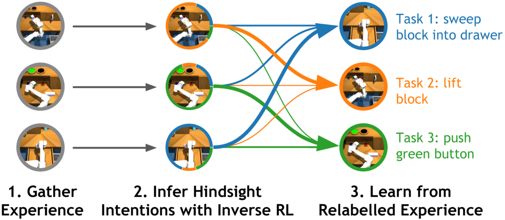
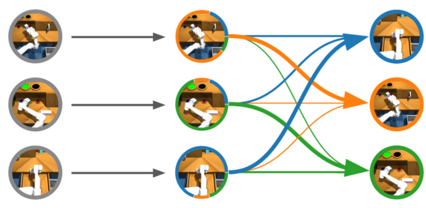
Figure 2: A number of recent multi-task RL algorithms organize experience
based on what task each piece of experience solved. This process of post-hoc
organization is closely related to hindsight relabeling and inverse RL, and lies
at the core of recent multi-task RL algorithms that are based on supervised
learning.

A number of recent algorithms can be viewed as reincarnations of this idea, with a twist. The twist is that finding good data becomes much easier in the multi-task setting. These works typically either operate directly in a multi-task setting or modify the single-task setting to look like one. As we increase the number of tasks, all experience becomes optimal for some task. We now view three recent papers through this lens:

Goal-conditioned imitation learning:[Savinov 2018, Ghosh 2019, Ding 2019, Lynch 2020] In a goal-reaching task our data distribution consists of both the states and actions, as well as the attempted goal. As a robot’s failure to reach a commanded goal is nonetheless a success for reaching the goal it actually reached, we can optimize the data distribution by replacing the originally commanded goals with the goals actually reached. Thus, the hindsight relabelling performed by goal-conditioned imitation learning [Savinov 2018, Ghosh 2019, Ding 2019, Lynch 2020] and hindsight experience replay [Andrychowicz 2017] can be viewed as optimizing a non-parametric data distribution. Moreover, goal-conditioned imitation can be viewed as simply doing supervised learning (a.k.a behavior cloning) on optimized data. Interestingly, when this goal-conditioned imitation procedure with relabeling is repeated iteratively, it can be shown that this is a convergent procedure for learning policies from scratch, even if no expert data is provided at all! [Ghosh 2018] This is particularly promising because it essentially provides us a technique for off-policy RL without explicitly requiring any bootstrapping or value function learning, significantly simplifying the algorithm and tuning process.

Reward-Conditioned Policies:[Kumar 2019, Srivastava 2019] Interestingly, we can the extend the insight discussed above to single-task RL, if we can view non-expert trajectories collected from sub-optimal policies as optimal supervision for some family of tasks. Of course, these sub-optimal trajectories may not maximize reward, but they are optimal for matching the reward of the given trajectory. Thus, we can modify the policy to be conditioned on a desired value of long-term reward (i.e., the return) and follow a similar strategy as goal-conditioned imitation learning: execute rollouts using this reward-conditioned policy by commanding a desired value of return, relabel the commanded return values to the observed returns, which gives us optimized data non-parametrically, and finally, run supervised learning on this optimized data. We show [Kumar 2019] that by simply optimizing the data in a non-parametric fashion via simple re-weighting schemes, we can obtain an RL method that is guaranteed to converge to the optimal policy and is simpler than most RL methods in that it does not require parametric return estimators which might be hard to tune.

Hindsight Inference for Policy Improvement:[Eysenbach 2020] While the connections between goal-reaching algorithms and dataset optimization are neat, until recently it was unclear how to apply similar ideas to more general multi-task settings, such as a discrete set of reward functions or sets of reward defined by varying (linear) combinations of bonus and penalty terms. To resolve this open question, we started with the intuition that optimizing the data distribution corresponds to answering the following question: “if you assume that your experience was optimal, what tasks were you trying to solve?” Intriguily, this is precisely the question that inverse RL answers. This suggests that we can simply use inverse RL to relabel data in arbitrary multi-task settings: inverse RL provides a theoretically grounded mechanism for sharing experience across tasks. This result is exciting for two reasons:

This result tells us how to apply similar relabeling ideas to more general multi-task settings. Our experiments showed that relabeling experience using inverse RL accelerates learning across a wide range of multi-task settings, and even outperformed prior goal-relabelling methods on goal-reaching tasks.
It turns out that relabeling with the goal actually reached is exactly equivalent to doing inverse RL with a certain sparse reward function. This result allows us to interpret previous goal-relabeling techniques as inverse RL, thus providing a stronger theoretical foundation for these methods. More generally, this result is exciting

Future Directions

In this article, we discussed how RL can be viewed as solving a sequence of standard supervised learning problems but using optimized (relabled) data. This success of deep supervised learning over the past decade might indicate that such approaches to RL may be easier to use in practice. While the progress so far is promising, there are several open questions. Firstly, what could be other (better) ways of obtaining optimized data? Does re-weighting or recombining existing experience induce bias in the learning process? How should the RL algorithm explore to obtain better data? Methods and analyses that make progress on this front are likely to also provide insights for algorithms derived from alternate perspectives on RL. Secondly, these methods might provide an easy way to carry over practical techniques as well as theoretical analyses from deep learning to RL, which are otherwise hard due to non-convex objectives (e.g., policy gradients) or mismatch in optimization and test-time objective (e.g., Bellman error and policy return). We are excited about several prospects these methods offer: improved practical RL algorithms, improved understanding of RL methods, etc.

We thank Allen Zhu, Shreyas Chaudhari, Sergey Levine, and Daniel Seita for feedback on this post.

This post is based on the following papers:

Ghosh, D., Gupta, A., Fu, J., Reddy, A., Devin, C., Eysenbach, B., & Levine,
S. (2019). Learning to Reach Goals via Iterated Supervised Learning
arXiv:1912.06088.
Eysenbach, B., Geng, X., Levine, S., & Salakhutdinov, R. (2020). Rewriting
History with Inverse RL: Hindsight Inference for Policy Improvement. NeurIPS 2020 (oral).
Kumar, A., Peng, X. B., & Levine, S. (2019). Reward-Conditioned Policies.
arXiv:1912.13465.

Our lower bound is technically an evidence lower bound, so coordinate ascent on it is equivalent to expectation maximization. ↩
While supervised learning is generally more stable than RL, iterated supervised learning may be less stable than supervised learning on a fixed dataset. ↩

This article was initially published on the BAIR blog, and appears here with the authors’ permission.

BAIR blog

AIhub is supported by:

Reinforcement learning is supervised learning on optimized data

Common Perspectives on RL

Optimization Perspective

Dynamic Programming Perspective

Supervised Learning Perspective

An RL objective that decouples the policy from data

Optimizing the Policy

Optimizing the Data Distribution

Viewing Prior Work through the Lens of Supervised Learning

Multi-Task Versions of the Supervised Learning Perspective

Future Directions

Related posts :

2024 AAAI / ACM SIGAI Doctoral Consortium interviews compilation

Interview with Andrews Ata Kangah: Localising illegal mining sites using machine learning and geospatial data

#NeurIPS social media round-up part 2

The Good Robot podcast: Machine vision with Jill Walker Rettberg

Five ways you might already encounter AI in cities (and not realise it)

#NeurIPS2024 social media round-up part 1

Congratulations to the #NeurIPS2024 award winners

Multi-agent path finding in continuous environments

↑