☰

ΑΙhub.org

Goodhart’s law, diversity and a series of seemingly unrelated toy problems

by BAIR blog

30 November 2020

share this:

By Aldo Pacchiano, Jack Parker-Holder, Luke Metz, and Jakob Foerster

Goodhart’s Law is an adage which states the following:

“When a measure becomes a target, it ceases to be a good measure.”

This is particularly pertinent in machine learning, where the source of many of our greatest achievements comes from optimizing a target in the form of a loss function. The most prominent way to do so is with stochastic gradient descent (SGD), which applies a simple rule, follow the gradient:

$\theta_{t+1} = \theta_t - \alpha \nabla_\theta \mathcal{L}(\theta_t)$

For some step size $\alpha$ . Updates of this form have led to a series of breakthroughs from computer vision to reinforcement learning, and it is easy to see why it is so popular: 1) it is relatively cheap to compute using backprop 2) it is guaranteed to locally reduce the loss at every step and finally 3) it has an amazing track record empirically.

However, we wouldn’t be writing this if SGD was perfect! In fact there are some negatives. Most importantly, there is an intrinsic bias towards ‘easy’ solutions (typically associated with high negative curvature). In some cases, two solutions with the same loss may be qualitatively different, and if one is easier to find then it is likely to be the only solution found by SGD. This has recently been referred to as a “shortcut” solution [1], examples of which are below:

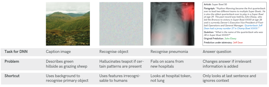
As we see, when classifying sheep, the network learns to use the green background to identify the sheep present. When instead it is provided with an image of sheep on a beach (which is an interesting prospect) then it fails altogether. Thus, the key question motivating our work is the following:

Question: How can we find a diverse set of different solutions?

Our answer to this is to follow eigenvectors of the Hessian (‘ridges’) with negative eigenvalues from a saddle, in what we call Ridge Rider (RR). There is a lot to unpack in that statement, so we will go into more detail in the following section.

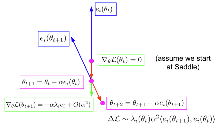
First, we assume we start at a saddle (green), where the norm of the gradient is zero. We compute the eigenvectors and eigenvalues of the Hessian, which solve the following:

$\mathcal{H}(\theta) e_i(\theta) = \lambda_i(\theta) e_i(\theta), |e_i| = 1$

And we follow the eigenvectors with negative eigenvalues, which we call ridges. We can follow these in both directions. As you see in the diagram, when we take a step along the ridge (in red) we reach a new point. Now the gradient is the step size multiplied by the eigenvalue and the eigenvector, because the eigenvector was of the Hessian. Now we re-compute the spectrum, and select the new ridge as the one with the highest inner product with the previous, to preserve the direction. We then take a step along a new ridge, to $\theta_{t+2}$ .

So why do we do about this? Well, in the paper we show that if the inner product between the new and the old ridge is greater than zero then we are theoretically guaranteed to improve our loss. What this means is, RR provides us with an orthogonal set of loss reducing directions. This is opposed to SGD, which will almost always follow just one.

The full picture

In the next diagram we show the full Ridge Rider algorithm.

We begin at a Maximally Invariant Saddle (MIS) that retains and respects all of the symmetries of the underlying problem. We branch, and select a ridge to follow, which we update until we reach a breaking point where we branch again. At this point we can choose whether to continue along the current path or select another ridge from the buffer. This is equivalent to choosing between breadth first search of depth first search. Finally the leaves of the tree are the solutions to our problem, each is uniquely defined by the fingerprint.

On the positive side, RR provides us with a set of orthogonal locally loss-reducing directions that can be used to span a tree of solutions. It essentially turns optimization into a search problem, which allows us to introduce new methods to use for finding solutions. We also benefit from the natural ordering and grouping scheme provided by the eigenvalues (Fingerprint).

However, of course, there are many obvious questions that naturally arise with this approach. Here we try to answer the FAQs:

Q: This seems expensive! Don’t you need loads of samples due to the high variance of Hessian?

A: Yes, that is fair! 🙁

Q: This seems expensive! Do you need to re-evaluate the full spectrum of the Hessian each timestep?

A: Actually no! We present an approximate version of RR using Hessian Vector Products. We will go into this next.

We use the Power/Lanczos method in GetRidges. In UpdateRidge, after each step along the ridge, we find the new $e_i, \lambda_i$ pair by minimizing:

$L(e_i, \lambda_i ; \theta) = |(1/\lambda_i) \mathcal{H}(\theta) e_i / |e_i| - e_i/|e_i| |^2$

We warm-start with the 1st-order approximation to $\lambda(\theta)$ , where $\theta', \lambda', e_i'$ are the previous values:

$\lambda_i(\theta) \approx \lambda_i' + e_i' \delta \mathcal{H} e_i' = \lambda_i' + e_i' (\mathcal{H}(\theta) - \mathcal{H}(\theta')) e_i'$

These terms only rely on Hessian vector products!

Q: This seems expensive! Don’t you need to evaluate hundreds or thousands of branches?

A: We actually don’t. We show in the paper that symmetries lead to repeated Eigenvalues, which reduces the number of branches we need to explore.

A symmetry, $\phi$ , of the loss function is a bijection on the parameter space such that

$\mathcal{L}_\theta = \mathcal{L}_{\phi(\theta)}, \quad \mbox{for all} \quad \theta \in \Theta$

We show that in the presence of symmetries, the Hessian has repeated eigenvalues. This means we only have to explore one from each set!

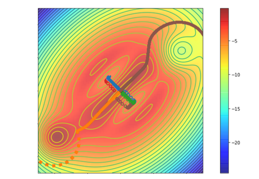
RR in action: An illustrative example

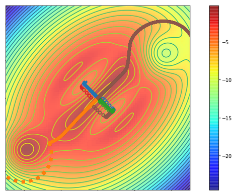
The Figure above shows a 2d cost surface, where we begin in the middle and want to reach the blue areas. SGD always gets stuck in the valleys which correspond to the locally steepest descent direction, this is shown by the circles. When running RR, the first ridge also follows this direction, as we see in blue and green. However, the second, orthogonal direction (brown and orange) avoids the local optima and reaches the high value regions.

Ridge Rider for Exploration in Reinforcement Learning

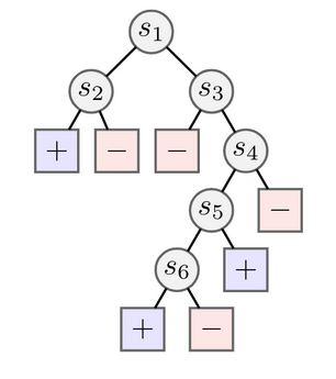
We tested RR in the tabular RL setting, where we sought to find diverse solutions to a tree-based exploration task. We generated trees like the one above, which has positive or negative rewards at the leaves. In this case we see it is much easier to find the positive reward on the left, corresponding to a policy which goes left at $s_1$ and left at $s_2$ . To find the solution at the bottom (going left from $s_6$ ) requires avoiding several negative rewards.

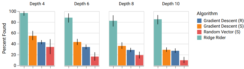
To rigorously evaluate RR, we generated 20 trees for four different depths, and ran the algorithm each time, comparing against Gradient Descent starting from random initializations or the MIS, and random vectors from the MIS. The results show that RR on average finds almost all the solutions, while the other methods fail to even find half.

In the paper we include additional ablations, and a first foray into sample-based RL. We encourage you to check it out.

Ridge Rider for Supervised Learning

We wanted to test the approximate RR algorithm in the simplest possible setting, which naturally brought us to MNIST, the canonical ML dataset! We used the approximate version to train a neural network with two 128-unit hidden layers, and surprisingly we were able to get 98% accuracy. This clearly isn’t a new SoTA for computer vision, but we think it is a nice result which shows the possible scalability of our algorithm.

Interestingly, it seems the individual ridges correspond to learning different features. In the next Figure, we show the performance for a classifier trained by following each ridge individually.

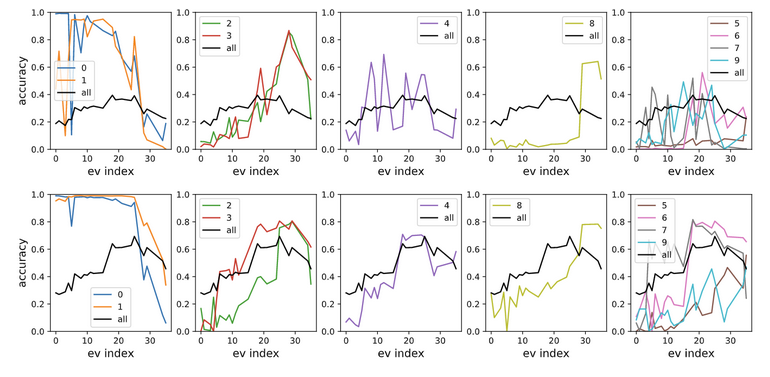
As we see, the earlier ridges correspond to learning 0 and 1, while the later ones learn to classify the digit 8.

This provides further evidence that the Hessian contains structure which may relate to causal information about the problem. Next we further develop this by looking at out-of-distribution generalization.

Ridge Rider for Out of Distribution Generalization

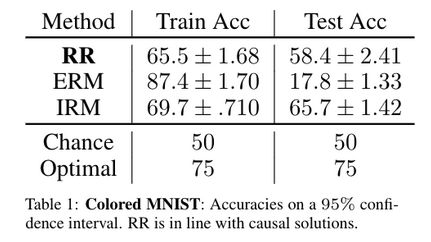
We tested RR on the colored MNIST dataset, from [2]. Colored MNIST was specifically designed to test causality, as each image is colored either red or green in a way that correlates strongly (but spuriously) with the class label. By construction, the label is more strongly correlated with the color than with the digit. Any algorithm purely minimizing training error will tend to exploit the color.

In the next Figure, we see that ERM (greedily optimizing the loss at training time) massively overfits the problem, and does poorly at test time. By contrast, RR achieves a respectable 58%, not too far from the 66% achieved by the state-of-the-art causal approach.

Ridge Rider for Zero-Shot Co-ordination

Finally, we consider the zero-shot co-ordination problem. In this setting, we wish to co-ordinate with a partner, but cannot see their policy in training. Instead, we can agree on a training strategy, for example — which ridge to follow.

We use an adapted version of the lever game from [3], shown below:

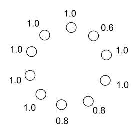
Recall from before that symmetries lead to repeated eigenvalues. This means the levers which share a payoff with others will have the same eigenvalue. Furthermore, the ordering of the ridges corresponding to repeated eigenvalues is inconsistent across different runs. Thus, we can only coordinate reliably on unique directions. We ran RR multiple times, and show the result for three independent runs below.

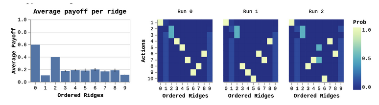
On the right, we see the first ridge is always the same action, which corresponds to the optimal zero-shot solution. The next two are a 50-50 bet on the two 0.8 ridges. The remaining ridges are largely a jumbled up mess, corresponding to the levers with symmetries.

Summary and Future Work

A gif speaks a thousand words:

Paper:

Ridge Rider: Finding Diverse Solutions by Following Eigenvectors of the Hessian.
Jack Parker-Holder, Luke Metz, Cinjon Resnick, Hengyuan Hu, Adam Lerer, Alistair Letcher, Alex Peysakhovich, Aldo Pacchiano, Jakob Foerster. NeurIPS 2020.
Paper Link

Code:

RL: https://bit.ly/2XvEmZy
ZS Co-ordination: https://bit.ly/308j2uQ
OOD Generalization: https://bit.ly/3gWeFsH

References:

[1] Robert Geirhos, Jörn-Henrik Jacobsen, Claudio Michaelis, Richard Zemel, Wieland Brendel, Matthias Bethge, Felix A. Wichmann (2020) Shortcut Learning in Deep Neural Networks.
[2] Martin Arjovsky, Léon Bottou, Ishaan Gulrajani, David Lopez-Paz (2019) Invariant Risk Minimization. Arxiv pre-print.
[3] Hengyuan Hu, Adam Lerer, Alex Peysakhovich, and Jakob Foerster. “Other-Play” for zero-shot coordination. International Conference on Machine Learning (ICML). 2020

This article was initially published on the BAIR blog, and appears here with the authors’ permission.