
ΑΙhub.org
Training on test inputs with amortized conditional normalized maximum likelihood

By Aurick Zhou
Current machine learning methods provide unprecedented accuracy across a range of domains, from computer vision to natural language processing. However, in many important high-stakes applications, such as medical diagnosis or autonomous driving, rare mistakes can be extremely costly, and thus effective deployment of learned models requires not only high accuracy, but also a way to measure the certainty in a model’s predictions. Reliable uncertainty quantification is especially important when faced with out-of-distribution inputs, as model accuracy tends to degrade heavily on inputs that differ significantly from those seen during training. In this blog post, we will discuss how we can get reliable uncertainty estimation with a strategy that does not simply rely on a learned model to extrapolate to out-of-distribution inputs, but instead asks: “given my training data, which labels would make sense for this input?”.
To illustrate how this can allow for more reasonable predictions on out-of-distribution data, consider the following example where we attempt to classify automobiles, where all the class 1 training examples are sedans and class 2 examples are large buses.
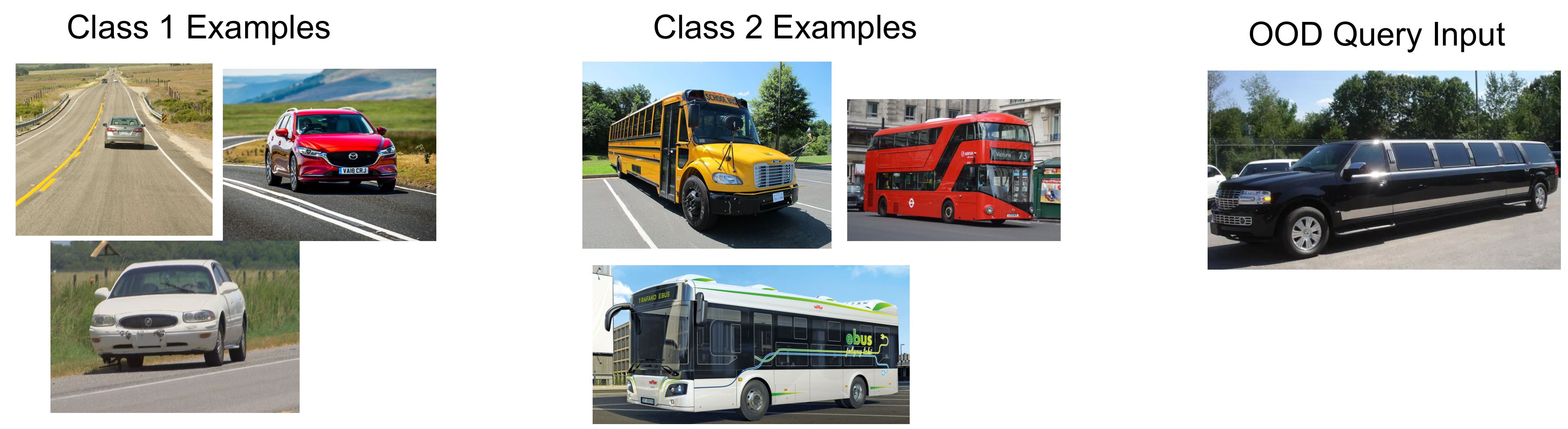
Figure 1: Given previously seen examples, it is uncertain what the label for the new query point should be. Different classifiers that work well on the training set can give different predictions on the query point.
A classifier could potentially fit the training labels correctly based on several different explanations; for example, it could notice that buses are all longer than sedans and classify accordingly, or it could perhaps pay attention to the height of the vehicle instead. However, if we try to simply extrapolate to an out-of-distribution image of a limousine, the classifier’s output could be unpredictable and arbitrary. A classifier based on length could note that the limousine is similar to the buses in its length and confidently predict class 2, while a classifier utilizing the height could confidently predict class 1. Based only on the training set, there is not enough information to accurately decide which class a limousine should fit into, so we would ideally want our classifier to indicate uncertainty instead of providing arbitrary confident predictions for either class. On the other hand, if we explicitly try to find models that explain each potential label, we would find reasonable explanations for either label, suggesting that we should be uncertain about predicting which class the limousine belongs to.
We can instantiate this reasoning with an algorithm that, for every possible label, explicitly updates the model to try to explain that label for the query point and combines the different models to obtain well-calibrated predictions for out-of-distribution inputs. In this blog post, we will motivate and introduce amortized conditional normalized maximum likelihood (ACNML), a practical instantiation of this idea that enables reliable uncertainty estimation with deep neural networks.
Conditional Normalized Maximum Likelihood
Our method extends a prediction strategy from the minimum description length (MDL) literature known as conditional normalized maximum likelihood (CNML),1 which has been studied for its theoretical properties, but is computationally intractable for all but the simplest problems. We will first review CNML and discuss how its predictions can lead to conservative uncertainty estimates. We will then describe our method, which allows for a practical application of CNML to obtain uncertainty estimates for deep neural networks.
The CNML distribution is derived from achieving a notion of minimax optimality, where we define a notion of regret for each label and choose the distribution that minimizes the worst case regret over labels. Given a training set  , a query input
  , and a set of potential models
  , we define the regret for each label to be the difference between the negative log-likelihood loss for our distribution and the loss under the model that best fits the training dataset together with the query point and label.
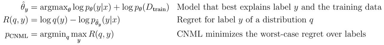
Intuitively, minimizing the worst case regret over labels then ensures our predictive distribution is conservative, as it cannot assign low probabilities to any labels that appear consistent with our training data, where consistency is determined by the model class.
The minimax optimal distribution given a particular input and training set  can be explicitly computed as follows:
- For each label
 , we append
  to our training set and compute the new optimal parameters
  for this modified training set.
 - Use to assign probability for that label.
- Since these probabilities will now sum to a number greater than 1, we normalize to obtain a valid distribution over labels.

CNML has the interesting property that it explicitly optimizes the model to make predictions on the query input, which can lead to more reasonable predictions than simply extrapolating using a model obtained only from the training set. It can also lead to more conservative predictions on out-of-distribution inputs, since it would be easier to fit different labels for out-of-distribution points without affecting performance on the training set.
We illustrate CNML with a 2-dimensional logistic regression example. We compare heatmaps of CNML probabilities with the maximum likelihood classifier to illustrate how CNML provides conservative uncertainty estimates on points away from the data. With this model class, CNML expresses uncertainty and assigns a uniform distribution to any query point where the dataset remains linearly separable (meaning there exists a linear decision boundary could correctly classify all data points) regardless of which label was assigned for the query point.
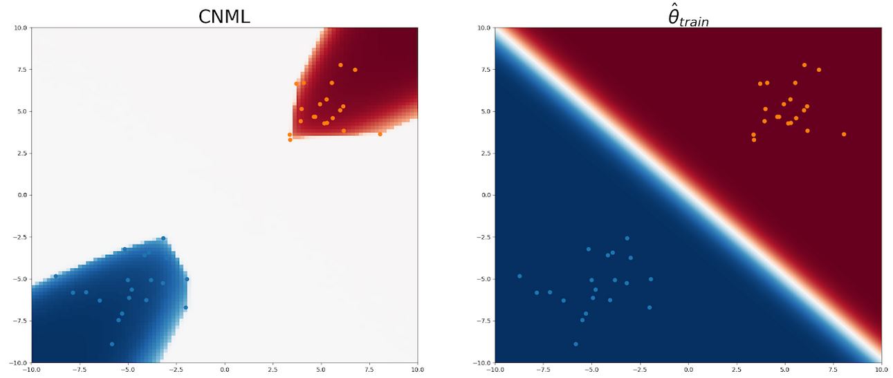
Figure 2: Here, we show the heatmap of CNML predictions (left) and the predictions of the training set MLE  (right). The training inputs are shown with blue (class 0) and orange (class 1) dots. Blue shading indicates that higher probability for class 0 on that input and red shading indicates higher probability to class 1, with darker colors indicating more confident predictions. We note that while the original classifier assigns confident predictions for most inputs, CNML assigns close to uniform for most points between the two clusters of training points, indicating high uncertainty about these ambiguous inputs.
We illustrate how CNML computes these probabilities by illustrating the base classifier predictions under parameters (the training set MLE), as well as  ,
,  , the parameters computed by CNML after assigning the labels 0 and 1 respectively to a query point.
We first consider an out-of-distribution query point far away from any of the training inputs (shown in pink in the bottom of the leftmost image). In the left image, we see the original decision boundary for confidently classifies the query point as class 0. In the middle, we see the decision boundary of  similarly classifies the query point as class 0. However, we see in the rightmost image that
  is able to confidently classify the query point as class 1. Since confidently predicts class 0 for the query point and confidently predicts class 1, CNML normalizes the two predictions to assign roughly equal probability to either label.
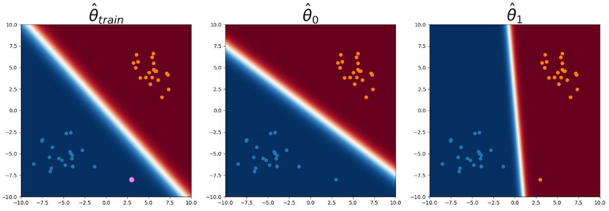
Figure 3: Query point shown in pink. Both and classify the query point as class 0, but is able to classify it as class 1.
On the other hand, for an in-distribution query point (again shown in pink) in the middle of the class 0 training inputs, no linear classifier can fit a label of 1 to the query point while still accurately fitting the rest of the training data, so the CNML distribution still confidently predicts class 0 on this query point.
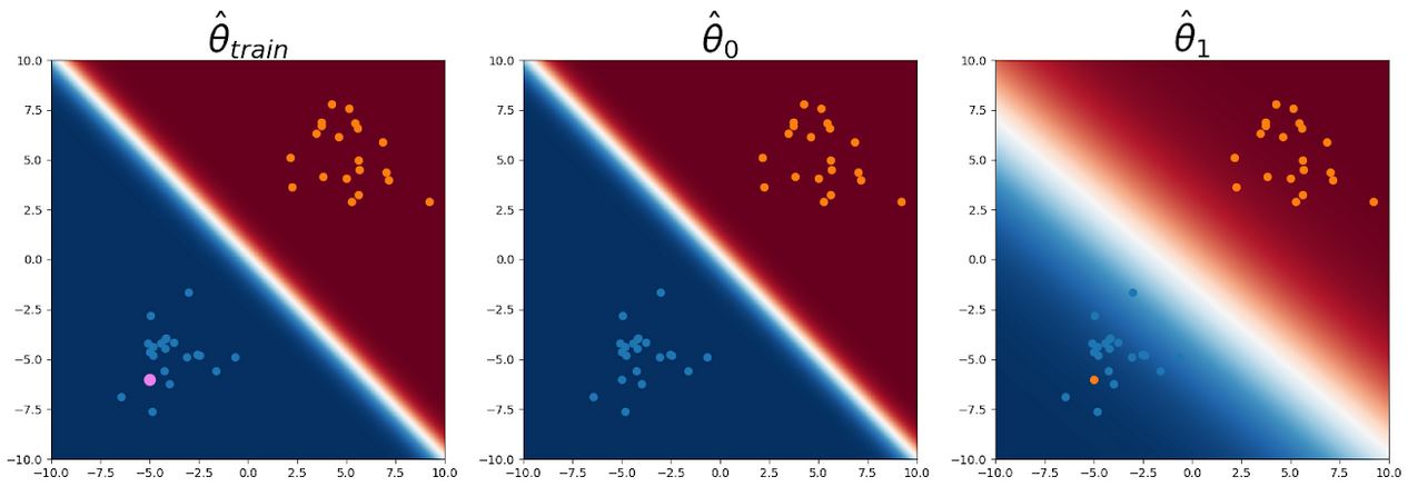
Figure 4: Query point shown in pink. All parameters are forced to classify the query point as class 0 since it is in the middle of the class 0 training points.
Controlling Conservativeness via Regularization
We see in Figure 2 that CNML probabilities are uniform on most of the input space, arguably being too conservative. In this case, the model class is in some sense too expressive, as linear predictors with large coefficients that can assign arbitrarily high probabilities to each label as long as the data remains linearly separable. This problem is exacerbated with even more expressive model classes like deep neural networks, which can potentially fit arbitrary labels. In order to have CNML give more useful predictions, we would need to constrain the allowed set of models to better reflect our notion of reasonable models.
To accomplish this, we generalize CNML to incorporate regularization via a prior term, resulting in conditional normalized maximum a posteriori (CNMAP) instead. Instead of computing maximum likelihood parameters for the training dataset and the new input and label, we compute maximum a posteriori (MAP) solutions instead, with the prior term  serving as a regularizer to limit the complexity of the selected model.

Going back to the logistic regression example, we add different levels of L2 regularization to the parameters (corresponding to Gaussian priors) and plot CNMAP probabilities in Figure 3 below. As regularization increases, CNML becomes less conservative, with the assigned probabilities transitioning much more smoothly as one moves away from the training points.
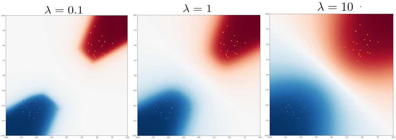
Figure 5: Heatmaps of CNMAP probabilities under varying amounts of regularization  . Increasing regularization leads to less conservative predictions.
Computational Intractability
While we see that CNML is able to provide conservative predictions for OOD inputs, computing CNML predictions requires retraining the model using the entire training set multiple times for each test input, which can be very computationally expensive. While explicitly computing CNML distributions was feasible in our logistic regression example with small datasets, it would be computationally intractable to compute CNML naively with datasets consisting of thousands of images and using deep convolutional neural networks, as retraining the model just once could already take many hours. Even initializing from the solution to the training set and finetuning for several epochs after adding the query input and label could still take several minutes per input, rendering it impractical to use with deep neural networks and large datasets.
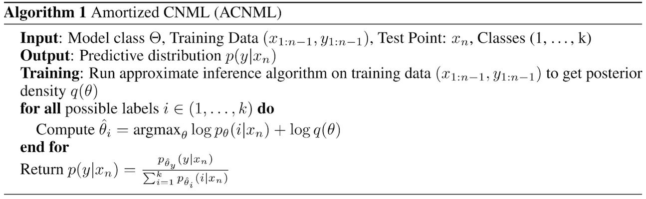
Amortized Conditional Normalized Maximum Likelihood
Since exactly computing CNML or CNMAP distributions is computationally infeasible in deep learning settings due to the need to optimize over large datasets for each new input and label, we need a tractable approximation. In our method, amortized conditional normalized maximum likelihood (ACNML), we utilize approximate Bayesian posteriors to capture necessary information about the training data in order to efficiently compute the MAP/MLE solutions for each datapoint. ACNML amortizes the costs of repeatedly optimizing over the training set by first computing an approximate Bayesian posterior, which serves as a compact approximation to the training losses.
CNMAP and Bayesian Posteriors
We note that the main computational bottleneck is the need to optimize over the entire training set for each query point. In order to sidestep this issue, we first show a relationship between the MAP parameters needed in CNMAP and Bayesian posterior densities:

Rather than computing optimal parameters for the new query point and the training set, we can reformulate CNMAP as optimizing over just the query point and a posterior density. With a uniform prior (equivalent to having no regularizer), we can recover the maximum likelihood parameters to perform CNML if desired.2
ACNML now utilizes approximate Bayesian inference to replace the exact Bayesian posterior density with a tractable density  . As many methods have been proposed for approximate Bayesian inference in deep learning, we can simply utilize any approximate posterior that provides tractable densities for ACNML, though we focus on Gaussian approximate posteriors for simplicity and computational efficiency. After computing the approximate posterior once during training, the test-time optimization procedure becomes much simpler, as we only need to optimize over our approximate posterior instead of the training set. When we instantiate ACNML and initialize from the MAP solution, we find that it typically takes only a handful of gradient updates to compute new (approximate) optimal parameters for each label, resulting in much faster test-time inference than a naive CNML instantiation that fine tunes using the whole training set.
In our paper, we analyze the approximation error incurred by using a particular Gaussian posterior in place of the exact training data likelihoods, and show that under certain assumptions, the approximation is accurate when the training set is large.
Experiments
We instantiate ACNML with two different Gaussian posterior approximations, SWAG-Diagonal and KFAC-Laplace and train models on the CIFAR-10 image classification dataset. To evaluate out-of-distribution performance, we then evaluate on the CIFAR-10 Corrupted datasets, which apply a diverse range of common image corruptions at different intensities, allowing us to see how well methods perform under varying levels of distribution shift. We compare against methods using Bayesian marginalization, which average predictions across different models sampled from the approximate posterior. We note that all methods provide very similar accuracy both in-distribution and out-of-distribution, so we focus on comparing uncertainty estimates.
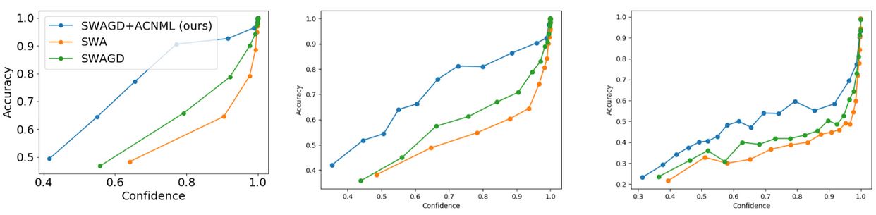
Figure 7: Reliability Diagrams comparing ACNML against the corresponding Bayesian model averaging method (SWAGD) and the MAP solution (SWA). ACNML generally predicts with lower confidence than other methods, leading to comparatively better uncertainty estimation as the data becomes more out-of-distribution.
We first examine ACNML’s predictions using reliability diagrams, which aggregate the test data points into buckets based on how confident the model’s predictions are, then plot the average confidence in a bucket against the actual accuracy of the predictions. These diagrams show the distribution of predicted confidences and can capture how effectively a model’s confidence reflects the actual uncertainty over the prediction.
As we would expect from our earlier discussion about CNML, we find that ACNML reliably gives more conservative (less confident) predictions than other methods, to the point where its predictions are actually underconfident on the in-distribution CIFAR10 test set where all methods provide very accurate predictions. However, on the out-of-distribution CIFAR10-C tasks where classifier accuracy degrades, ACNML’s conservativeness provides much more reliable confidence estimates, while other methods tend to be severely overconfident.
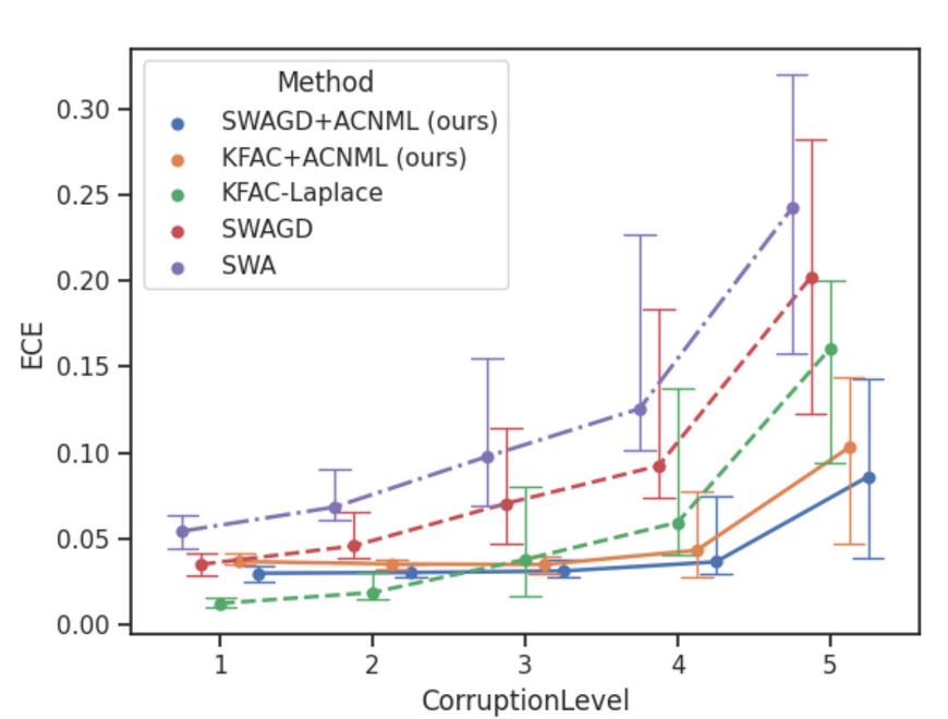
Figure 8: ECE comparisons: We compare instantiations of ACNML with two different approximate posteriors against their Bayesian counterparts.
We quantitatively measure calibration using the Expected Calibration Error, which uses the same buckets as the reliability diagrams and computes the average calibration error (absolute difference between average confidence and accuracy within the bucket) over all buckets. We see that ACNML instantiations provide much better calibration than their Bayesian counterparts and the deterministic baseline as the corruption intensities increase and the data becomes more out-of-distribution.
Discussion
In this post, we discussed how we can obtain reliable uncertainty estimates on out-of-distribution data by explicitly optimizing on the data we wish to make predictions on instead of relying on trained models to extrapolate from the training data. We then showed that this can be done concretely with the CNML prediction strategy, a scheme that has been studied theoretically but is computationally intractable to apply in practice. Finally we presented our method, ACNML, a practical approximation to CNML that enables reliable uncertainty estimation with deep neural networks. We hope that this line of work will help enable broader applicability of large scale machine learning systems, especially in safety-critical domains where uncertainty estimation is a necessity.
We thank Sergey Levine and Dibya Ghosh for providing valuable feedback on this post.
This post is based on this following paper:
- Aurick Zhou, Sergey Levine.
Amortized Conditional Normalized Maximum Likelihood.
- For additional background on MDL and CNML, we refer to the following textbook. The particular variant of CNML used here is referred to as CNML-3 in the text, and as sNML-1 in Roos et al. ↩
- Despite referring to maximum likelihood in the name, ACNML actually approximates the CNMAP procedure, with CNML being a special case of CNMAP by using a uniform prior as regularizer. In practice, due to the over-conservativeness of CNML mentioned before, we will use non-uniform priors (as used by the Bayesian deep learning methods we build off of). ↩
This article was initially published on the BAIR blog, and appears here with the authors’ permission.

AUAI is supported by: