Representational aspects of depth and conditioning in normalizing flows

By Viraj Mehta and Andrej Risteski

The promise of unsupervised learning lies in its potential to take advantage of cheap and plentiful unlabeled data to learn useful representations or generate high-quality samples. For the latter task, neural network-based generative models have recently enjoyed a lot of success in producing realistic images and text. Two major paradigms in deep generative modeling are generative adversarial networks (GANs) and normalizing flows. When successfully scaled up and trained, both can generate high-quality and diverse samples from high-dimensional distributions. The training procedure for GANs involves min-max (saddle-point) optimization, which is considerably more difficult than standard loss minimization, leading to problems like mode dropping.

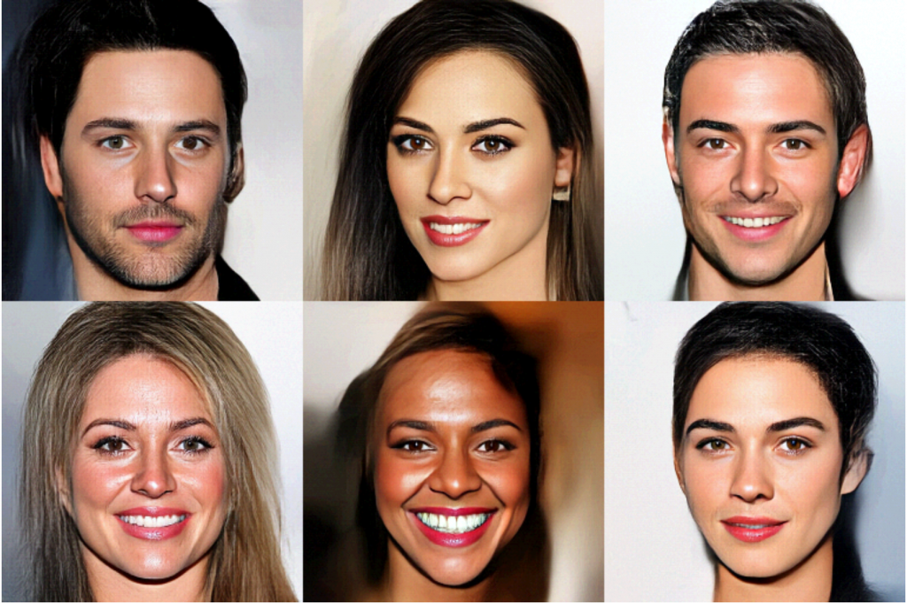
Normalizing flows [1] have been proposed as an alternative type of generative model which allows not only efficient sampling but also training via maximum likelihood through a closed-form computation of the likelihood function. They are written as pushforwards of a simple distribution (typically a Gaussian) through an invertible transformation , typically parametrized as a composition of simple invertible transformations. The main reason for this parametrization is the change-of-variables formula: if is a random variable sampled from a known base distribution (typically a standard multivariate normal), is invertible and differentiable, and then

Here, is the Jacobian of .

Normalizing flows are trained by maximizing the likelihood using gradient descent. However, in practice, training normalizing flows runs into difficulties as well: models which produce good samples typically need to be extremely deep — which comes with accompanying vanishing/exploding gradient problems. A very related problem is that they are often poorly conditioned. Data like images are often inherently lower-dimensional than the ambient space, the map from low dimensional data to high dimensional latent variables can be difficult to invert and therefore train.

In our recent work [2], we tackle representational questions around depth and conditioning of normalizing flows—first for general invertible architectures, then for a particular common architecture—where the normalizing flow is a composition of so-called affine couplings.

Depth Bound on General Invertible Architectures

The most fundamental restriction of the normalizing flow paradigm is that each layer needs to be invertible. We ask whether this restriction has any ‘cost’ in terms of the size, and in particular the depth, of the model. Here we’re counting depth in terms of the number of the invertible transformations that make up the flow. A requirement for large depth would explain training difficulties due to exploding (or vanishing) gradients.

A natural way of formalizing this question is by exhibiting a distribution which is easy to model for an unconstrained generator network but hard for a shallow normalizing flow. Precisely, we ask: is there a probability distribution that can be represented by a shallow generator with a small number of parameters that could not be approximately represented by a shallow composition of invertible transformations?

We demonstrate that such a distribution exists. Specifically, we show that

Theorem: For every k, s.t. and any parameterized family of compositions of Lipschitz invertible transformations with parameters per transformation and at most transformations, there exists a generator with depth and parameters s.t the pushforward of a Gaussian through cannot be approximated in either KL or Wasserstein-1 distance by a network in this family.

The result above is extremely general: it only requires a bound on the number of parameters per transformation in the parametrization of the normalizing flow and Lipschitzness of these maps. As such it easily includes common choices used in practice like affine couplings with at most parameters per layer or invertible feedforward networks, where each intermediate layer is of dimension and the nonlinearity is invertible (e.g. leaky ReLU). On the flip side, for possible architectures with a large number of parameters per transformation, this theorem gives a (possibly loose) lower bound of a small number of transformations.

Proof Sketch: The generator for our construction approximates a mixture of Gaussians with means placed uniformly randomly on a -dimensional sphere in the ambient space. We will use the probabilistic method to show there is a family of such mixtures, s.t. each pair of members in this family are far apart (say, in Wasserstein distance). Furthermore, by an epsilon net discretization argument we can count how many “essentially” distinct invertible Lipschitz networks there are. If the number of mixtures in the family is much larger than the size of the epsilon net, at least one mixture must be far from all invertible networks.

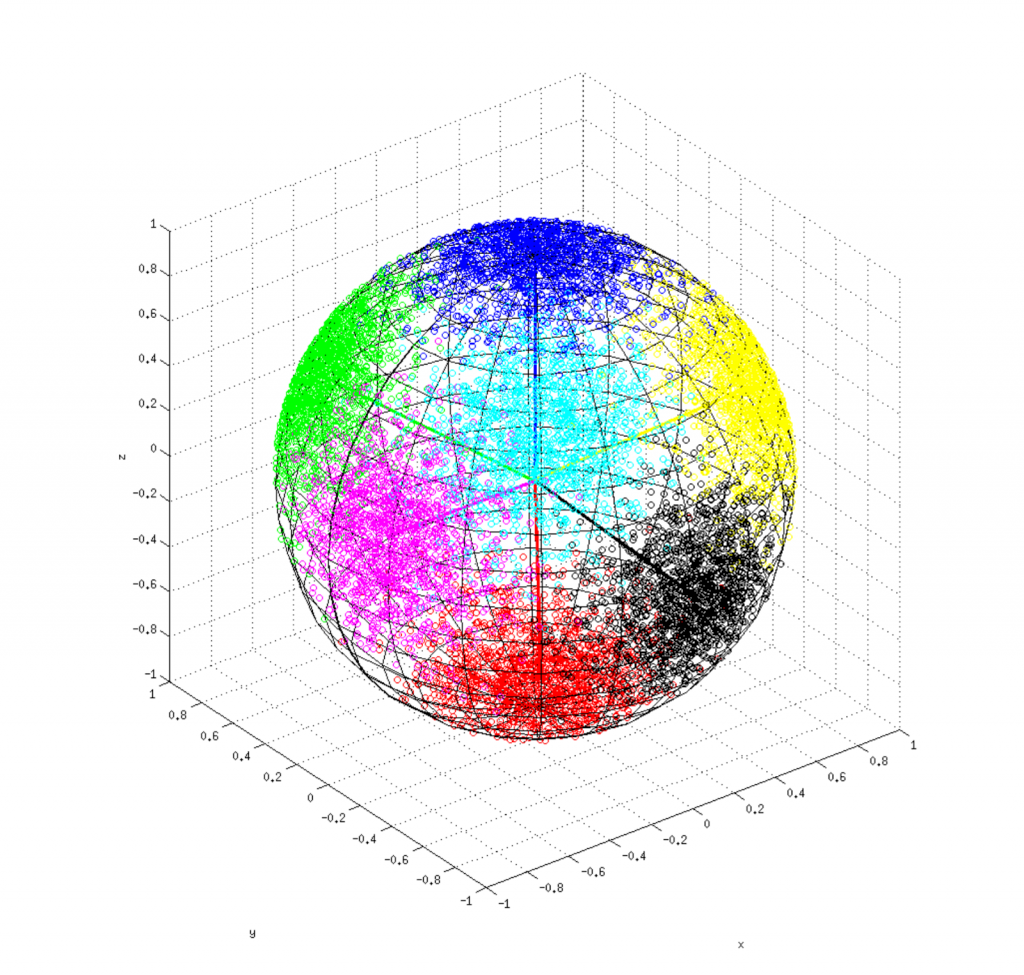
The family of mixtures is constructed by choosing the means for the components uniformly at random on a sphere. It’s well known that randomly chosen points on a unit sphere will, with high probability, have constant pairwise distance. Similarly, coding-theoretic arguments (used to prove the so-called Gilbert-Varshamov bound) can be used to show that selecting -tuples of those means will, with high probability, ensure that each pair of -tuples is such that the average pair of means is at constant distance. This suffices to ensure the Wasserstein distance between pairs of mixtures is large. ∎

Results for Affine Couplings

Affine Couplings [3] are one of the most common transformations in scalable architectures for normalizing flows. An affine coupling is a map such that for some partition into a set containing approximately half of the coordinates and it’s complement,

for some scaling and translation functions (typically parameterized by neural networks) and . Clearly, an affine coupling block only transforms one partition of the coordinates at a time by an affine function while leaving the other partition intact. It’s easy to see that an affine coupling is invertible if each coordinate of is invertible. Moreover, the Jacobian of this function is

In particular it’s lower triangular, so we can calculate the determinant in linear time by multiplying the diagonal elements (in general determinants take time to compute). This allows us to efficiently compute likelihoods and their gradients for SGD on large models via the change of variables formula.
These affine coupling blocks are stacked, often while changing the part of the partition that is updated or more generally, permuting the elements in between the application of the coupling.

Effect of the Choice of Partition on Representational Power

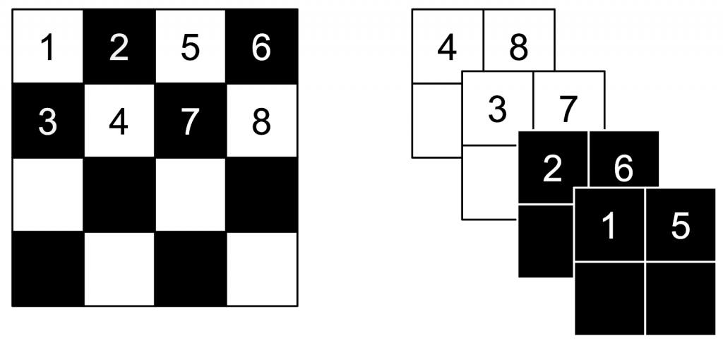
The choice of partition is often somewhat ad-hoc and involves domain knowledge (e.g. for image datasets, a typical choice is a checkerboard pattern or a channel-wise partition). In fact, some recent approaches like GLOW [4] try to “learn” permutations to apply between each pair of affine couplings. (Technically, since a permutation is a discrete object, in [4] the authors learn a 1×1 convolutions instead.)

While ablation experiments provide definite evidence that including learned 1×1 convolutions is beneficial for modeling image data in practice, it’s unclear whether this effect is from increased modeling power or algorithmic effects — and even less so how to formally quantify it. In this section, we come to a clear understanding of the representational value of adding this flexibility in partitioning. We knew from GLOW that adding these partitions helped. Now we know why!

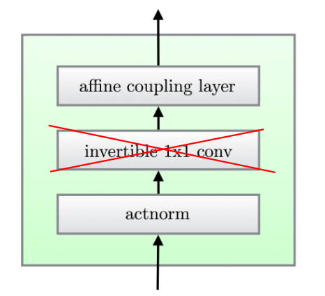
We formalize the representational question as follows: how many affine couplings with a fixed partition are needed to simulate an arbitrary linear map? Since a linear map is more general than a 1×1 convolution, if it’s possible to do so with a small (say constant) number of affine couplings, we can simulate any affine coupling-based normalizing flow including 1×1 convolutions by one that does not include them which is merely a constant factor larger.

Concretely, we consider linear functions of the form

for matrices and diagonal matrices . The right hand side is precisely a composition of affine coupling blocks with linear maps with a fixed partition (the parts of the input that are being updated alternate). We show the following result:

Theorem: To represent an arbitrary invertible , must be at most 24. Additionally, there exist invertible matrices such that .

Proof sketch: The statement hopefully reminds the reader of the standard LU decomposition — the twist of course being that the matrices on the right-hand side have a more constrained structure than merely being triangular. Our proof starts with the existence of a decomposition for every matrix.

We first show that we can construct an arbitrary permutation (up to sign) using at most 21 alternating matrices of the desired form. The argument is group theoretic: we use the fact that a permutation decomposes into a composition of two permutations of order 2, which must be disjoint products of swaps and show that swapping elements can be implemented “in parallel” using several partitioned matrices of the type we’re considering.

Next, we show that we can produce an arbitrary triangular matrix with our partitioned matrices. We use similar techniques as above to reduce the matrix to a regular system of block linear equations which we can then solve. Our upper bound comes from just counting the total number of matrices required for these operations: the 21 for the permutation and 13 for each triangular matrix (upper and lower), giving a total of 47 required matrices. ∎

To reiterate the takeaway: a GLOW-style linear layer in between affine couplings could in theory make your network between 5 and 47 times smaller while representing the same function. We now have a precise understanding of the value of that architectural choice!

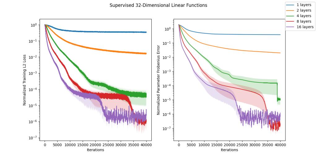
We also verified empirically in the figure below how well these linear models would fit randomly chosen (i.e. with iid Gaussian entries) linear functions. It seems empirically that at least for this ensemble our upper bound is loose and we can fit the functions well without using the full 47 layers. Closing this gap is an interesting problem for future work.

Universal Approximation with Poorly Conditioned Networks

In our earlier result on the depth of invertible networks, we assumed that our network was Lipschitz and therefore well-conditioned. A natural question is then, if we remove this requirement, how powerful is the resulting class of models? In particular, we ask: are poorly conditioned affine coupling-based normalizing flows universal approximators as they are used in practice?

Curiously, this question has in fact not been answered in prior work. In a very recent work [5], it was shown that if we allow for padding of our data with extra dimensions that take a constant value 0, affine couplings are universal approximators. (Note, this kind of padding clearly results in a singular Jacobian — as the value in the added dimensions is constant.) The idea for why padding helps is that these extra dimensions are used as a “scratch pad” for the computation the network is performing. Another recent work [6] gives a proof of universal approximation for affine couplings assuming arbitrary permutations in between the layers are allowed (ala Glow) and a partition separating dimensions from the other. However, in practice, these models are trained using a roughly half-half split and often without linear layers in between couplings (which already works quite well). We prove that none of these architectural modifications to affine couplings are necessary for universal approximation and additionally suggest a trade-off between the conditioning of the model and the quality of its approximation. Concretely, we show:

Theorem: For any bounded and absolutely continuous distribution over and any , there exists a 3-layer affine coupling with maps represented by feedforward ReLU networks such that , where is the pushforward of a standard Gaussian through .

We note that the construction for the theorem trades off quality of approximation () with conditioning: the smallest singular value of the Jacobian in the construction for our theorem above will scale like — thus suggesting that if we want to use affine couplings as universal approximators, conditioning may be an issue even if we don’t pad with a constant value for the added dimensions like prior works — which obviously results in a singular Jacobian.

Proof sketch: The proof is based on two main ideas.

The first is a deep result from optimal transport, Brenier’s theorem, which for sufficiently “regular” distributions over guarantees an invertible map , s.t. the pushforward of the Gaussian through equals . This reduces our problem to approximating using a sequence of affine couplings.

The difficulty in approximating is the fact that affine couplings are only allowed to change one part of the input, and in a constrained way. The trick we use to do this without a “scratchpad” to store intermediate computation as in prior works is to instead hide information in the “low order bits” of the other partition. For details, refer to our paper. ∎

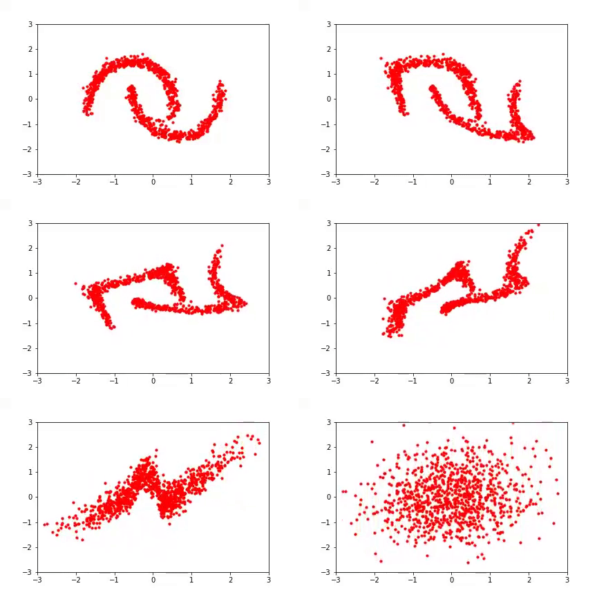
Finally, on the experimental front, we wanted to experiment with how padding affects the conditioning of a learned model. We considered synthetic 2d datasets (see figure below) and found that padding with zeros resulted in a very poorly conditioned model which produced poor samples, as might be expected. We also considered a type of padding which is reasonable but for which we have no theory — namely, to use iid Gaussian samples as values for the added dimensions (in this case, the resulting Jacobians are not prima facie singular, and the model can still use them as a “scratch pad”). While we have no result that this in any formal sense can result in better-conditioned networks, we found that in practice it frequently does and it also results in better samples. This seems like a very fruitful direction for future research. Finally, without padding, the model produces samples of middling quality and has a condition number in between that of zero and Gaussian padding.

Conclusions

Normalizing flows are one of the most popular generative models across various domains, though we still have a relatively narrow understanding of their relative pros and cons compared to other models. We show in this work that there are fundamental tradeoffs between depth and conditioning and representational power of this type of function. Though we have cleared up considerably the representational aspects of these models, the algorithmic and statistical questions are still wide open. We hope that this work guides both users of flows and theoreticians as to the fine-grained properties of flows as compared to other generative models.

Bibliography

[1] Rezende and Mohamed, 2015, Variational Inference with Normalizing Flows, ICML 2015

[2] Koehler, Mehta, and Risteski, 2020, Representational aspects of depth and conditioning in normalizing flows, Under Submission.

[3] Dinh, Sohl-Dickstein, and S. Bengio, 2016, Density estimation using Real NVP, ICLR 2016

[4] Kingma and Dhariwal, 2018, GLOW: Generative flow with 1×1 convolutions, NeurIPS 2018

[5] Huang, Dinh, and Courville, 2020, Augmented Normalizing Flows: Bridging the Gap Between Generative Flows and Latent Variable Models

[6] Teshima, Ishikawa, Tojo, Oono, Ikeda, and Sugiyama, 2020, Coupling-based Invertible Neural Networks Are Universal Diffeomorphism Approximators, NeurIPS 2020

This article was initially published on the ML@CMU blog and appears here with the authors’ permission.

ML@CMU

ML@CMU