
ΑΙhub.org
A learning theoretic perspective on local explainability
By Vaishnavh Nagarajan and Jeffrey Li
Fig 1: A formal relationship between interpretability and complexity. Going from left to right, we consider increasingly complex functions. As the complexity increases, local linear explanations can approximate the function only in smaller and smaller neighborhoods. These neighborhoods, in other words, need to become more and more disjoint as the function becomes more complex. Indeed, we quantify “disjointedness” of the neighborhoods via a term denoted by  and relate it to the complexity of the function class, and subsequently, its generalization properties.
Introduction
There has been a growing interest in interpretable machine learning (IML), towards helping users better understand how their ML models behave. IML has become a particularly relevant concern especially as practitioners aim to apply ML in important domains such as healthcare [Caruana et al., ’15], financial services [Chen et al., ’18], and scientific discovery [Karpatne et al., ’17].
While much of the work in IML has been qualitative and empirical, in our recent ICLR21 paper, we study how concepts in interpretability can be formally related to learning theory. At a high level, the connection between these two fields seems quite natural. Broadly, one can consider there to be a trade-off between notions of a model’s interpretability and its complexity. That is, as a model’s decision boundary gets more complicated (e.g., compare a sparse linear model vs. a neural network) it is harder in a general sense for a human to understand how it makes decisions. At the same time, learning theory commonly analyzes relationships between notions of complexity for a class of functions (e.g., the number of parameters required to represent those functions) and the functions’ generalization properties (i.e., their predictive accuracy on unseen test data). Therefore, it is natural to suspect that, through some appropriate notion of complexity, one can establish connections between interpretability and generalization.
How do we establish this connection? First, IML encompasses a wide range of definitions and problems, spanning both the design of inherently interpretable models as well as post-hoc explanations for black-boxes (e.g. including but not limited to approximation [Riberio et al., ’16], counterfactual [Dhurandhar et al., ’18], and feature importance-based explanations [Lundberg & Lee, ’17]). In our work, we focus on a notion of interpretability that is based on the quality of local approximation explanations. Such explanations are a common and flexible post-hoc approach for IML, used by popular methods such as LIME [Riberio et al., ’16] and MAPLE [Plumb et al., ‘18] which we’ll briefly outline later in the blog. We then answer two questions that relate this notion of local explainability to important statistical properties of the model:
- Performance Generalization: How can a model’s predictive accuracy on unseen test data be related to the interpretability of the learned model?
- Explanation Generalization: We look at a novel statistical problem that arises in a growing subclass of local approximation algorithms (such as MAPLE and RL-LIM [Yoon et al., ‘19]). Since these algorithms learn explanations by fitting them on finite data, the explanations may not necessarily fit unseen data well. Hence, we ask, what is the quality of those explanations on unseen data?
In what follows, we’ll first provide a quick introduction to local explanations. Then, we’ll motivate and answer our two main questions by discussing a pair of corresponding generalization guarantees that are in terms of how “accurate” and “complex” the explanations are. Here, the “complexity” of the local explanations corresponds to how large of a local neighborhood the explanations span (the larger the neighborhood, the lower the complexity — see Fig 1 for a visualization). For question (1), this results in a bound that roughly captures the idea that an easier-to-locally-approximate  enjoys better performance generalization. For question (2), our bound tells us that, when the explanations can accurately fit all the training data that fall within large neighborhoods, the explanations are likely to fit unseen data better. Finally, we’ll examine our insights in practice by verifying that these guarantees capture non-trivial relationships in a few real-world datasets.
Local Explainability
Local approximation explanations operate on a basic idea: use a model from a simple family (like a linear model) to locally mimic a model from a more complex family (like a neural network model). Then, one can directly inspect the approximation (e.g. by looking at the weights of the linear model). More formally, for a given black-box model  , the explanation system produces at any input
  , a ”simple” function
  that approximates in a local neighborhood around
  . Here, we assume
  (the complex model class) and
  (the simple model class).
As an example, here’s what LIME (Local Interpretable Model-agnostic Explanations) does. At any point , in order to produce the corresponding explanation  , LIME would sample a bunch of perturbed points in the neighborhood around and label them using the complex function
  . It would then learn a simple function that fits the resulting dataset. One can then use this simple function to better understand how behaves in the locality around .
Performance Generalization
Our first result is a generalization bound on the squared error loss of the function . Now, a typical generalization bound would look something like
![\[\text{TestLoss}(f) \le \text{TrainLoss}(f) + \sqrt{ \frac{\text{Complexity}(\mathcal{F})}{\text{# of training examples}} }\]](https://aihub.org/wp-content/ql-cache/quicklatex.com-062c223ddc4f84239f25668ac8abe986_l3.png "Rendered by QuickLaTeX.com")
where the bound is in terms of how well fits the training data, and also how “complex” the function class  is. In practice though, can often be a very complex class, rendering these bounds too large to be meaningful.
Yet while is complex, what if the function might itself have been picked from a subset of that is in some way much simpler? For example, this is the case in neural networks trained by gradient descent [Zhang et al., ‘17, Neyshabur et al., ‘15]). Capturing this sort of simplicity could lead to more interesting bounds that (a) aren’t as loose and/or (b) shed insight into what meaningful properties of can influence how well it generalizes. While there are many different notions of simplicity that different learning theory results have studied, here we are interested in quantifying simplicity in terms of how “interpretable” is, and relate that to generalization.
To state our result, imagine that we have a training set  sampled from the data distribution
  . Then, we show the following bound on the test-time squared error loss:
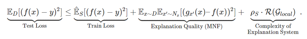
Let’s examine these terms one by one.
Train Loss: The first term, as is typical of many generalization bounds, is simply the training error of on  .
.
Explanation Quality (MNF): The second term captures a notion of how interpretable is, measuring how accurate the set of local explanations  is with a quantity that we call the “mirrored neighborhood fidelity” (MNF). This metric is actually a slight modification of a standard notion of local explanation quality used in IML literature, called neighborhood fidelity (NF) [Riberio et al., ’16; Plumb et al., ‘18]. More concretely, we explain how MNF and NF are calculated below in Fig 2.
Fig 2. How MNF is calculated: We use orange to denote “source points” (where explanations are generated) and teal to denote “target points” (where approximation error is computed). To compute the inner expectation for MNF, we sample a single target point  . Then, we sample a source point
  from a “neighborhood” distribution
  (typically a distribution centered at ). We then measure how well is approximated at by the explanation generated at . Averaging over and , we define
 ![\text{MNF} = \mathbb{E}_{x \sim D} \mathbb{E}_{x' \sim N_{x}}[(g_{x'}(x) - f(x))^2]](https://aihub.org/wp-content/ql-cache/quicklatex.com-42edbd884d9393af02bd1320338045c2_l3.png "Rendered by QuickLaTeX.com") . To get NF, we simply need to swap and in the innermost term:
. To get NF, we simply need to swap and in the innermost term: ![\text{NF} = \mathbb{E}_{x \sim D} \mathbb{E}_{x' \sim N_{x}}[(g_{x}(x') - f(x'))^2]](https://aihub.org/wp-content/ql-cache/quicklatex.com-7c9deff297417e38e5e36de41ab35a45_l3.png "Rendered by QuickLaTeX.com") .
.
While notationally the differences between MNF and the standard notion of NF are slight, there are some noteworthy differences and potential (dis)advantages of using MNF over NF from an interpretability point of view. At a high level, we argue that MNF offers more robustness (when compared to NF) to any potential irregular behavior of off the manifold of the data distribution. We discuss this in greater detail in the full paper.
Complexity of Explanation System: Finally, the third and perhaps the most interesting term measures how complex the infinite set of explanation functions  is. As it turns out, this system of explanations , which we will call , has a complexity that can be nicely decomposed into two factors. One factor, namely
  , corresponds to the (Rademacher) complexity of the simple local class
  , which is going to be a very small quantity, much smaller than the complexity of . Think of this factor as typically scaling linearly with the number of parameters for and also with the dataset size
  as
as  . The second factor is , and is what we call the “neighborhood disjointedness” factor. This factor lies between
 ![[1, \sqrt{m}]](https://aihub.org/wp-content/ql-cache/quicklatex.com-7d9aa4799795935b718333389c52cb82_l3.png "Rendered by QuickLaTeX.com") and is defined by how little overlap there is between the different local neighborhoods specified for each of the training datapoints in . When there is absolutely no overlap, can be as large as
and is defined by how little overlap there is between the different local neighborhoods specified for each of the training datapoints in . When there is absolutely no overlap, can be as large as  , but when all these neighborhoods are exactly the same, equals
  .
.
Implications of the overall bound: Having unpacked all the terms, let us take a step back and ask: assuming that has fit the training data well (i.e., the first term is small), when are the other two terms large or small? We visualize this in Fig 1. Consider the case where MNF can be made small by approximating by on very large neighborhoods (Fig 1 left). In such a case, the neighborhoods would overlap heavily, thus keeping small as well. Intuitively, this suggests good generalization when is “globally simple”. On the other hand, when is too complex, then we need to either shrink the neighborhoods or increase the complexity of to keep MNF small. Thus, one would either suffer from MNF or exploding, suggesting bad generalization. In fact, when is as large as , the bound is “vacuous” as the complexity term no longer decreases with the dataset size , suggesting no generalization!
Explanation Generalization
We’ll now turn to a different, novel statistical question which arises when considering a number of recent IML algorithms. Here we are concerned with how well explanations learned from finite data generalize to unseen data.
To motivate this question more clearly, we need to understand a key difference between canonical and finite-sample-based IML approaches. In canonical approaches (e.g. LIME), at different values of , the explanations  are learned by fitting on a fresh bunch of points
  from a (user-defined) neighborhood distribution
  (see Fig 3, top). But a growing number of approaches such as MAPLE and RL-LIM learn their explanations by fitting on a “realistic” dataset drawn from (rather than from an arbitrary distribution) and then re-weighting the datapoints in depending on a notion of their closeness to (see Fig 3, bottom).
Now, while the canonical approaches effectively train on an infinite dataset  , recent approaches train on only that finite dataset (reused for every
  ).
).
Using a realistic has certain advantages (as motivated in this blog post), but on the flip side, since is finite, it can potentially result in a severe chance of overfitting (we visualize this in Fig 3 right). This makes it valuable to seek a guarantee on the approximation error of on test data (“Test MNF”) in terms of its fit on the training data (“Train MNF”). In our paper, we derive such a result below:
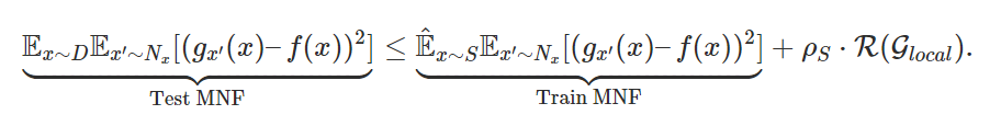
As before, what this bound implies is that when the neighborhoods have very little overlap, there is poor generalization. This indeed makes sense: if the neighborhoods are too tiny, any explanation would have been trained on a very small subset of that falls within its neighborhood. Thus the fit of won’t generalize to other neighboring points.
Fig 3. Difference between canonical local explanations (a) vs. finite-sample-based explanations (b and c): On the top panel (a), we visualize how one would go about generating explanations for different source points in a canonical method like LIME. In the bottom panels (b and c), we visualize the more recent approaches where one uses (and reuses) a single dataset for each explanation. Crucially, to learn an explanation at a particular source point, these procedures correspondingly re-weight this common dataset (visualized by the orange square boxes which are more opaque for points closer to each source point). In panel (b), the common dataset is large enough that it leads to good explanations; but in panel (c), the dataset is too small that the explanations do not generalize well to their neighborhoods.
Experiments
While our theoretical results offer insights that make sense qualitatively, we also want to make a case empirically that they indeed capture meaningful relationships between the quantities involved. Particularly, we explore this for neural networks trained on various regression tasks from the UCI suite and in the context of the “explanation generalization” bound. That is we learn explanations to fit a finite dataset by minimizing Train MNF, and then evaluate what Test MNF is like. Here, there are two important relationships we empirically establish:
- Dependence on : Given that our bounds may be vacuous for large
 , does this quantity actually scale well in practice (i.e. less than
  )? Indeed, we observe that we can find reasonably large choices of the neighborhood size
  without causing Train MNF to become too high (somewhere around
  in Fig 4 bottom) and for which we can also achieve a reasonably small
  (Fig 4 top).
 - Dependence on neighborhood size: Do wider neighborhoods actually lead to improved generalization gaps? From Fig 4 bottom, we do observe that as the neighborhood width increases, TrainMNF and TestMNF overall get closer to each other, indicating that the generalization gap decreases (Fig 4 bottom).
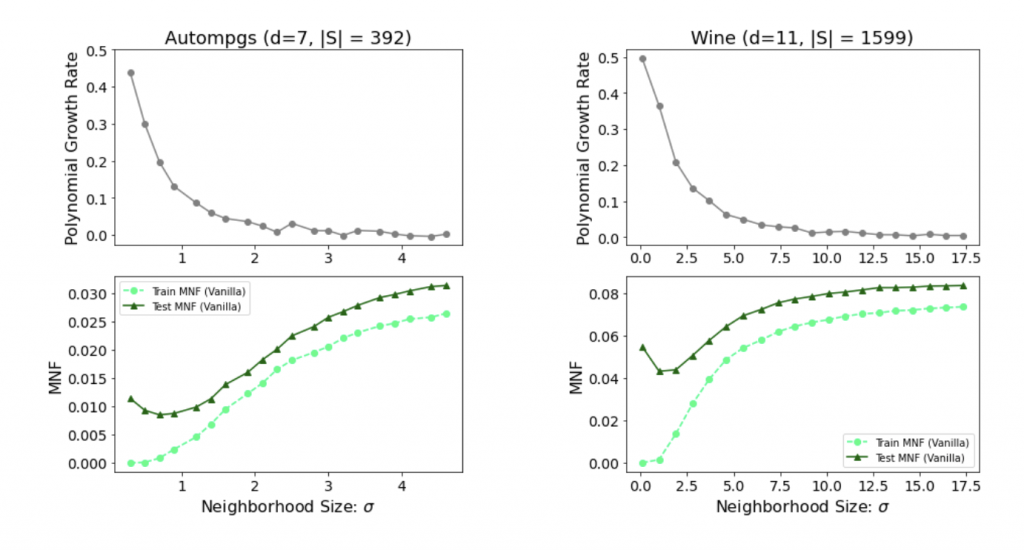
Fig 4. Empirical study of our bounds For various neighborhood widths , in the top, we plot the approximate exponent of ‘s polynomial growth rate i.e., the exponent  in
in  . Below, we plot train/test MNF. We observe a tradeoff here: increasing results in better values of but hurts the MNF terms.
Conclusion
We have shown how a model’s local explainability can be formally connected to some of its various important statistical properties. One direction for future work is to consider extending these ideas to high-dimensional datasets, a challenging setting where our current bounds become prohibitively large. Another direction would be to more thoroughly explore these bounds in the context of neural networks, for which researchers are in search of novel types of bounds [Zhang et al., ‘17; Nagarajan and Kolter ‘19].
Separately, when it comes to the interpretability community, it would be interesting to explore the advantages/disadvantages of evaluating and learning explanations via MNF rather than NF. As discussed here, MNF appears to have reasonable connections to generalization, and as we show in the paper, it may also promise more robustness to off-manifold behavior.
To learn more about our work, check out our upcoming ICLR paper. Moreover, for a broader discussion about IML and some of the most pressing challenges in the field, here is a link to a recent white paper we wrote.
References
Jeffrey Li, Vaishnavh Nagarajan, Gregory Plumb, and Ameet Talwalkar, 2021, “A Learning Theoretic Perspective on Local Explainability“, ICLR 2021.
Rich Caruana, Yin Lou, Johannes Gehrke, Paul Koch, Marc Sturm, and Noemie Elhadad, 2015, “Intelligible models for healthcare: Predicting pneumonia risk and hospital 30-day readmission.” ACM SIGKDD, 2015.
Chaofan Chen, Kancheng Lin, Cynthia Rudin, Yaron Shaposhnik, Sijia Wang, and Tong Wang, 2018, “An interpretable model with globally consistent explanations for credit risk.” NeurIPS 2018 Workshop on Challenges and Opportunities for AI in Financial Services: the Impact of Fairness, Explainability, Accuracy, and Privacy, 2018.
Anuj Karpatne, Gowtham Atluri, James H. Faghmous, Michael Steinbach, Arindam Banerjee, Auroop Ganguly, Shashi Shekhar, Nagiza Samatova, and Vipin Kumar, 2017, “Theory-guided data science: A new paradigm for scientific discovery from data.” IEEE Transactions on Knowledge and Data Engineering, 2017.
Marco Tulio Ribeiro, Sameer Singh, and Carlos Guestrin, 2016, “Why should I trust you?: Explaining the predictions of any classifier.” ACM SIGKDD, 2016.
Scott M. Lundberg, and Su-In Lee, 2017, “A unified approach to interpreting model predictions.” NeurIPS, 2017.
Amit Dhurandhar, Pin-Yu Chen, Ronny Luss, Chun-Chen Tu, Paishun Ting, Karthikeyan Shanmugam, and Payel Das, 2018, “Explanations based on the Missing: Towards Contrastive Explanations with Pertinent Negatives” NeurIPS, 2018.
Jinsung Yoon, Sercan O. Arik, and Tomas Pfister, 2019, “RL-LIM: Reinforcement learning-based locally interpretable modeling”, arXiv 2019 1909.12367.
Gregory Plumb, Denali Molitor and Ameet S. Talwalkar, 2018, “Model Agnostic Supervised Local Explanations“, NeurIPS 2018.
Vaishnavh Nagarajan and J. Zico Kolter, 2019, “Uniform convergence may be unable to explain generalization in deep learning”, NeurIPS 2019
Behnam Neyshabur, Ryota Tomioka, Nathan Srebro, 2015, “In Search of the Real Inductive Bias: On the Role of Implicit Regularization in Deep Learning”, ICLR 2015 Workshop.
Chiyuan Zhang, Samy Bengio, Moritz Hardt, Benjamin Recht, Oriol Vinyals, 2017, “Understanding deep learning requires rethinking generalization”, ICLR’ 17.
Valerie Chen, Jeffrey Li, Joon Sik Kim, Gregory Plumb, and Ameet Talwalkar, 2021, “Towards Connecting Use Cases and Methods in Interpretable Machine Learning“, arXiv 2021 2103.06254.
This article was initially published on the ML@CMU blog and appears here with the authors’ permission.

AUAI is supported by: