Should I use offline RL or imitation learning?

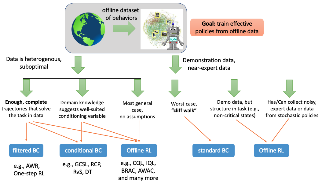
Figure 1: Summary of our recommendations for when a practitioner should BC and various imitation learning style methods, and when they should use offline RL approaches.

By Aviral Kumar, Ilya Kostrikov, Sergey Levine

Offline reinforcement learning allows learning policies from previously collected data, which has profound implications for applying RL in domains where running trial-and-error learning is impractical or dangerous, such as safety-critical settings like autonomous driving or medical treatment planning. In such scenarios, online exploration is simply too risky, but offline RL methods can learn effective policies from logged data collected by humans or heuristically designed controllers. Prior learning-based control methods have also approached learning from existing data as imitation learning: if the data is generally “good enough,” simply copying the behavior in the data can lead to good results, and if it’s not good enough, then filtering or reweighting the data and then copying can work well. Several recent works suggest that this is a viable alternative to modern offline RL methods.

This brings about several questions: when should we use offline RL? Are there fundamental limitations to methods that rely on some form of imitation (behavior cloning (BC), conditional BC, filtered BC) that offline RL addresses? While it might be clear that offline RL should enjoy a large advantage over imitation learning when learning from diverse datasets that contain a lot of suboptimal behavior, we will also discuss how even cases that might seem BC-friendly can still allow offline RL to attain significantly better results. Our goal is to help explain when and why you should use each method and provide guidance to practitioners on the benefits of each approach. Figure 1 concisely summarizes our findings and we will discuss each component.

Methods for learning from offline data

Let’s start with a brief recap of various methods for learning policies from data that we will discuss. The learning algorithm is provided with an offline dataset , consisting of trajectories generated by some behavior policy. Most offline RL methods perform some sort of dynamic programming (e.g., Q-learning) updates on the provided data, aiming to obtain a value function. This typically requires adjusting for distributional shift to work well, but when this is done properly, it leads to good results.

On the other hand, methods based on imitation learning attempt to simply clone the actions observed in the dataset if the dataset is good enough, or perform some kind of filtering or conditioning to extract useful behavior when the dataset is not good. For instance, recent work filters trajectories based on their return, or directly filters individual transitions based on how advantageous these could be under the behavior policy and then clones them. Conditional BC methods are based on the idea that every transition or trajectory is optimal when conditioned on the right variable. This way, after conditioning, the data becomes optimal given the value of the conditioning variable, and in principle we could then condition on the desired task, such as a high reward value, and get a near-optimal trajectory. For example, a trajectory that attains a return of is optimal if our goal is to attain return (RCPs, decision transformer); a trajectory that reaches goal is optimal for reaching (GCSL, RvS). Thus, one can perform perform reward-conditioned BC or goal-conditioned BC, and execute the learned policies with the desired value of return or goal during evaluation. This approach to offline RL bypasses learning value functions or dynamics models entirely, which can make it simpler to use. However, does it actually solve the general offline RL problem?

What we already know about RL vs imitation methods

Perhaps a good place to start our discussion is to review the performance of offline RL and imitation-style methods on benchmark tasks. In the figure below, we review the performance of some recent methods for learning from offline data on a subset of the D4RL benchmark.

Table 1: Dichotomy of empirical results on several tasks in D4RL. While imitation-style methods (decision transformer, %BC, one-step RL, conditional BC) perform at par with and can outperform offline RL methods (CQL, IQL) on the locomotion tasks, these methods simply break down on the more complex maze navigation tasks.

Observe in the table that while imitation-style methods perform at par with offline RL methods across the span of the locomotion tasks, offline RL approaches vastly outperform these methods (except, goal-conditioned BC, which we will discuss towards the end of this post) by a large margin on the antmaze tasks. What explains this difference? As we will discuss in this blog post, methods that rely on imitation learning are often quite effective when the behavior in the offline dataset consists of some complete trajectories that perform well. This is true for most replay-buffer style datasets, and all of the locomotion datasets in D4RL are generated from replay buffers of online RL algorithms. In such cases, simply filtering good trajectories, and executing the mode of the filtered trajectories will work well. This explains why %BC, one-step RL and decision transformer work quite well. However, offline RL methods can vastly outperform BC methods when this stringent requirement is not met because they benefit from a form of “temporal compositionality” which enables them to learn from suboptimal data. This explains the enormous difference between RL and imitation results on the antmazes.

Offline RL can solve problems that conditional, filtered or weighted BC cannot

To understand why offline RL can solve problems that the aforementioned BC methods cannot, let’s ground our discussion in a simple, didactic example. Let’s consider the navigation task shown in the figure below, where the goal is to navigate from the starting location A to the goal location D in the maze. This is directly representative of several real-world decision-making scenarios in mobile robot navigation and provides an abstract model for an RL problem in domains such as robotics or recommender systems. Imagine you are provided with data that shows how the agent can navigate from location A to B and how it can navigate from C to E, but no single trajectory in the dataset goes from A to D. Obviously, the offline dataset shown below provides enough information for discovering a way to navigate to D: by combining different paths that cross each other at location E. But, can various offline learning methods find a way to go from A to D?

Figure 2: Illustration of the base case of temporal compositionality or stitching that is needed find optimal trajectories in various problem domains.

It turns out that, while offline RL methods are able to discover the path from A to D, various imitation-style methods cannot. This is because offline RL algorithms can “stitch” suboptimal trajectories together: while the trajectories in the offline dataset might attain poor return, a better policy can be obtained by combining good segments of trajectories (A→E + E→D = A→D). This ability to stitch segments of trajectories temporally is the hallmark of value-based offline RL algorithms that utilize Bellman backups, but cloning (a subset of) the data or trajectory-level sequence models are unable to extract this information, since such no single trajectory from A to D is observed in the offline dataset!

Why should you care about stitching and these mazes? One might now wonder if this stitching phenomenon is only useful in some esoteric edge cases or if it is an actual, practically-relevant phenomenon. Certainly stitching appears very explicitly in multi-stage robotic manipulation tasks and also in navigation tasks. However, stitching is not limited to just these domains — it turns out that the need for stitching implicitly appears even in tasks that do not appear to contain a maze. In practice, effective policies would often require finding an “extreme” but high-rewarding action, very different from an action that the behavior policy would prescribe, at every state and learning to stitch such actions to obtain a policy that performs well overall. This form of implicit stitching appears in many practical applications: for example, one might want to find an HVAC control policy that minimizes the carbon footprint of a building with a dataset collected from distinct control policies run historically in different buildings, each of which is suboptimal in one manner or the other. In this case, one can still get a much better policy by stitching extreme actions at every state. In general this implicit form of stitching is required in cases where we wish to find really good policies that maximize a continuous value (e.g., maximize rider comfort in autonomous driving; maximize profits in automatic stock trading) using a dataset collected from a mixture of suboptimal policies (e.g., data from different human drivers; data from different human traders who excel and underperform under different situations) that never execute extreme actions at each decision. However, by stitching such extreme actions at each decision, one can obtain a much better policy. Therefore, naturally succeeding at many problems requires learning to either explicitly or implicitly stitch trajectories, segments or even single decisions, and offline RL is good at it.

The next natural question to ask is: Can we resolve this issue by adding an RL-like component in BC methods? One recently-studied approach is to perform a limited number of policy improvement steps beyond behavior cloning. That is, while full offline RL performs multiple rounds of policy improvement untill we find an optimal policy, one can just find a policy by running one step of policy improvement beyond behavioral cloning. This policy improvement is performed by incorporating some sort of a value function, and one might hope that utilizing some form of Bellman backup equips the method with the ability to “stitch”. Unfortunately, even this approach is unable to fully close the gap against offline RL. This is because while the one-step approach can stitch trajectory segments, it would often end up stitching the wrong segments! One step of policy improvement only myopically improves the policy, without taking into account the impact of updating the policy on the future outcomes, the policy may fail to identify truly optimal behavior. For example, in our maze example shown below, it might appear better for the agent to find a solution that decides to go upwards and attain mediocre reward compared to going towards the goal, since under the behavior policy going downwards might appear highly suboptimal.

Figure 3: Imitation-style methods that only perform a limited steps of policy improvement may still fall prey to choosing suboptimal actions, because the optimal action assuming that the agent will follow the behavior policy in the future may actually not be optimal for the full sequential decision making problem.

Is offline RL useful when stitching is not a primary concern?

So far, our analysis reveals that offline RL methods are better due to good “stitching” properties. But one might wonder, if stitching is critical when provided with good data, such as demonstration data in robotics or data from good policies in healthcare. However, in our recent paper, we find that even when temporal compositionality is not a primary concern, offline RL does provide benefits over imitation learning.

Offline RL can teach the agent what to “not do”. Perhaps one of the biggest benefits of offline RL algorithms is that running RL on noisy datasets generated from stochastic policies can not only teach the agent what it should do to maximize return, but also what shouldn’t be done and how actions at a given state would influence the chance of the agent ending up in undesirable scenarios in the future. In contrast, any form of conditional or weighted BC which only teach the policy “do X”, without explicitly discouraging particularly low-rewarding or unsafe behavior. This is especially relevant in open-world settings such as robotic manipulation in diverse settings or making decisions about patient admission in an ICU, where knowing what to not do very clearly is essential. In our paper, we quantify the gain of accurately inferring “what not to do and how much it hurts” and describe this intuition pictorially below. Often obtaining such noisy data is easy — one could augment expert demonstration data with additional “negatives” or “fake data” generated from a simulator (e.g., robotics, autonomous driving), or by first running an imitation learning method and creating a dataset for offline RL that augments data with evaluation rollouts from the imitation learned policy.

Figure 4: By leveraging noisy data, offline RL algorithms can learn to figure out what shouldn’t be done in order to explicitly avoid regions of low reward, and how the agent could be overly cautious much before that.

Is offline RL useful at all when I actually have near-expert demonstrations? As the final scenario, let’s consider the case where we actually have only near-expert demonstrations — perhaps, the perfect setting for imitation learning. In such a setting, there is no opportunity for stitching or leveraging noisy data to learn what not to do. Can offline RL still improve upon imitation learning? Unfortunately, one can show that, in the worst case, no algorithm can perform better than standard behavioral cloning. However, if the task admits some structure then offline RL policies can be more robust. For example, if there are multiple states where it is easy to identify a good action using reward information, offline RL approaches can quickly converge to a good action at such states, whereas a standard BC approach that does not utilize rewards may fail to identify a good action, leading to policies that are non-robust and fail to solve the task. Therefore, offline RL is a preferred option for tasks with an abundance of such “non-critical” states where long-term reward can easily identify a good action. An illustration of this idea is shown below, and we formally prove a theoretical result quantifying these intuitions in the paper.

Figure 5: An illustration of the idea of non-critical states: the abundance of states where reward information can easily identify good actions at a given state can help offline RL — even when provided with expert demonstrations — compared to standard BC, that does not utilize any kind of reward information,

So, when is imitation learning useful?

Our discussion has so far highlighted that offline RL methods can be robust and effective in many scenarios where conditional and weighted BC might fail. Therefore, we now seek to understand if conditional or weighted BC are useful in certain problem settings. This question is easy to answer in the context of standard behavioral cloning, if your data consists of expert demonstrations that you wish to mimic, standard behavioral cloning is a relatively simple, good choice. However this approach fails when the data is noisy or suboptimal or when the task changes (e.g., when the distribution of initial states changes). And offline RL may still be preferred in settings with some structure (as we discussed above). Some failures of BC can be resolved by utilizing filtered BC — if the data consists of a mixture of good and bad trajectories, filtering trajectories based on return can be a good idea. Similarly, one could use one-step RL if the task does not require any form of stitching. However, in all of these cases, offline RL might be a better alternative especially if the task or the environment satisfies some conditions, and might be worth trying at least.

Conditional BC performs well on a problem when one can obtain a conditioning variable well-suited to a given task. For example, empirical results on the antmaze domains from recent work indicate that conditional BC with a goal as a conditioning variable is quite effective in goal-reaching problems, however, conditioning on returns is not (compare Conditional BC (goals) vs Conditional BC (returns) in Table 1). Intuitively, this “well-suited” conditioning variable essentially enables stitching — for instance, a navigation problem naturally decomposes into a sequence of intermediate goal-reaching problems and then stitch solutions to a cleverly chosen subset of intermediate goal-reaching problems to solve the complete task. At its core, the success of conditional BC requires some domain knowledge about the compositionality structure in the task. On the other hand, offline RL methods extract the underlying stitching structure by running dynamic programming, and work well more generally. Technically, one could combine these ideas and utilize dynamic programming to learn a value function and then obtain a policy by running conditional BC with the value function as the conditioning variable, and this can work quite well (compare RCP-A to RCP-R here, where RCP-A uses a value function for conditioning; compare TT+Q and TT here)!

Empirical results comparing offline RL and BC

In our discussion so far, we have already studied settings such as the antmazes, where offline RL methods can significantly outperform imitation-style methods due to stitching. We will now quickly discuss some empirical results that compare the performance of offline RL and BC on tasks where we are provided with near-expert, demonstration data.

Figure 6: Comparing full offline RL (CQL) to imitation-style methods (One-step RL and BC) averaged over 7 Atari games, with expert demonstration data and noisy-expert data. Empirical details here.

In our final experiment, we compare the performance of offline RL methods to imitation-style methods on an average over seven Atari games. We use conservative Q-learning (CQL) as our representative offline RL method. Note that naively running offline RL (“Naive CQL (Expert)”), without proper cross-validation to prevent overfitting and underfitting does not improve over BC. However, offline RL equipped with a reasonable cross-validation procedure (“Tuned CQL (Expert)”) is able to clearly improve over BC. This highlights the need for understanding how offline RL methods must be tuned, and at least, in part explains the poor performance of offline RL when learning from demonstration data in prior works. Incorporating a bit of noisy data that can inform the algorithm of what it shouldn’t do, further improves performance (“CQL (Noisy Expert)” vs “BC (Expert)”) within an identical data budget. Finally, note that while one would expect that while one step of policy improvement can be quite effective, we found that it is quite sensitive to hyperparameters and fails to improve over BC significantly. These observations validate the findings discussed earlier in the blog post. We discuss results on other domains in our paper, that we encourage practitioners to check out.

Discussion and takeaways

In this blog post, we aimed to understand if, when and why offline RL is a better approach for tackling a variety of sequential decision-making problems. Our discussion suggests that offline RL methods that learn value functions can leverage the benefits of stitching, which can be crucial in many problems. Moreover, there are even scenarios with expert or near-expert demonstration data, where running offline RL is a good idea. We summarize our recommendations for practitioners in Figure 1, shown right at the beginning of this blog post. We hope that our analysis improves the understanding of the benefits and properties of offline RL approaches.

This blog post is primarily based on the paper:

When Should Offline RL Be Preferred Over Behavioral Cloning?
Aviral Kumar*, Joey Hong*, Anikait Singh, Sergey Levine [arxiv].
In International Conference on Learning Representations (ICLR), 2022.

In addition, the empirical results discussed in the blog post are taken from various papers, in particular from RvS and IQL.

This article was initially published on the BAIR blog, and appears here with the authors’ permission.

BAIR blog

BAIR blog