ΑΙhub.org
Optimizing LLM test-time compute involves solving a meta-RL problem
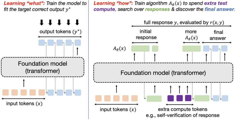 Figure 1: Training models to optimize test-time compute and learn “how to discover” correct responses, as opposed to the traditional learning paradigm of learning “what answer” to output.
By Amrith Setlur, Yuxiao Qu, Matthew Yang, Lunjun Zhang, Virginia Smith, Aviral Kumar
The major strategy to improve large language models (LLMs) thus far has been to use more and more high-quality data for supervised fine-tuning (SFT) or reinforcement learning (RL). Unfortunately, it seems this form of scaling will soon hit a wall, with the scaling laws for pre-training plateauing, and with reports that high-quality text data for training maybe exhausted by 2028, particularly for more difficult tasks, like solving reasoning problems which seems to require scaling current data by about 100x to see any significant improvement. The current performance of LLMs on problems from these hard tasks remains underwhelming (see example). There is thus a pressing need for data-efficient methods for training LLMs that extend beyond data scaling and can address more complex challenges. In this post, we will discuss one such approach: by altering the LLM training objective, we can reuse existing data along with more test-time compute to train models to do better.
Current LLMs are trained on “what” to answer
The predominant principle for training models today is to supervise them into producing a certain output for an input. For instance, supervised fine-tuning attempts to match direct output tokens given an input akin to imitation learning and RL fine-tuning trains the response to optimize a reward function that is typically supposed to take the highest value on an oracle response. In either case, we are training the model to produce the best possible approximation to ![]() it can represent. Abstractly, this paradigm trains models to produce a single input-output mapping, which works well when the goal is to directly solve a set of similar queries from a given distribution, but fails to discover solutions to out-of-distribution queries. A fixed, one-size-fits-all approach cannot adapt to the task heterogeneity effectively. We would instead want a robust model that is able to generalize to new, unseen problems by trying multiple approaches and seeking information to different extents, or expressing uncertainty when it is fully unable to fully solve a problem. How can we train models to satisfy these desiderata?
it can represent. Abstractly, this paradigm trains models to produce a single input-output mapping, which works well when the goal is to directly solve a set of similar queries from a given distribution, but fails to discover solutions to out-of-distribution queries. A fixed, one-size-fits-all approach cannot adapt to the task heterogeneity effectively. We would instead want a robust model that is able to generalize to new, unseen problems by trying multiple approaches and seeking information to different extents, or expressing uncertainty when it is fully unable to fully solve a problem. How can we train models to satisfy these desiderata?
Learning “how to answer” can generalize beyond
To address the above issue, one emerging idea is to allow models to use test-time compute to find “meta” strategies or algorithms that can help them understand “how” to arrive at a good response. If you are new to test-time compute check out these papers, this excellent overview talk by Sasha Rush, and the NeurIPS tutorial by Sean Welleck et al. Implementing meta strategies that imbue a model with the capability of running a systematic procedure to arrive at an answer should enable extrapolation and generalization to input queries of different complexities at test time. For instance, if a model is taught what it means to use the Cauchy-Schwarz inequality, it should be able to invoke it at the right time on both easy and hard proof problems (potentially by guessing its usage, followed by a trial-and-error attempt to see if it can be applied in a given problem). In other words, given a test query, we want models to be capable of executing strategies that involve several atomic pieces of reasoning (e.g., several generation and verification attempts; several partially-completed solutions akin to search; etc) which likely come at the cost of spending more tokens. See Figure 2 for an example of two different strategies to attack a given problem. How can we train models to do so? We will formalize this goal into a learning problem and solve it via ideas from meta RL.

Figure 2: Examples of two algorithms and the corresponding stream of tokens generated by each algorithm. This includes tokens that are used to fetch relevant information from the model weights, plan the proof outline, verify intermediate results, and revise if needed. The first algorithm (left) generates an initial solution, verifies its correctness and revises if needed. The second algorithm (right) generates multiple solution strategies at once, and runs through each of them in a linear fashion before choosing the most promising strategy.
Formulating learning “how” as an objective
For every problem ![]() , say we have a reward function
, say we have a reward function ![]() that we can query on any output stream of tokens
that we can query on any output stream of tokens ![]() . For e.g., on a math reasoning problem
. For e.g., on a math reasoning problem ![]() , with token output stream
, with token output stream ![]() , reward
, reward ![]() can be one that checks if some subsequence of tokens contains the correct answer. We are only given the dataset of training problems
can be one that checks if some subsequence of tokens contains the correct answer. We are only given the dataset of training problems ![]() , and consequently the set of reward functions
, and consequently the set of reward functions ![]() . Our goal is to achieve high rewards on the distribution of test problems
. Our goal is to achieve high rewards on the distribution of test problems ![]() , which are unknown apriori. The test problems can be of different difficulty compared to train problems.
, which are unknown apriori. The test problems can be of different difficulty compared to train problems.
For an unknown distribution of test problems ![]() , and a finite test-time compute budget
, and a finite test-time compute budget ![]() , we can learn an algorithm
, we can learn an algorithm ![]() in the inference compute-constrained class of test-time algorithms
in the inference compute-constrained class of test-time algorithms ![]() learned from the dataset of training problems
learned from the dataset of training problems ![]() . Each algorithm in this class takes as input the problem
. Each algorithm in this class takes as input the problem ![]() , and outputs a stream of tokens. In Figure 2, we give some examples to build intuition for what this stream of tokens can be. For instance,
, and outputs a stream of tokens. In Figure 2, we give some examples to build intuition for what this stream of tokens can be. For instance, ![]() could consist of tokens that first correspond to some attempt at problem
could consist of tokens that first correspond to some attempt at problem ![]() , then some verification tokens which predict the correctness of the attempt, followed by some refinement of the initial attempt (if verified to be incorrect), all stitched together in a “linear” fashion. Another algorithm
, then some verification tokens which predict the correctness of the attempt, followed by some refinement of the initial attempt (if verified to be incorrect), all stitched together in a “linear” fashion. Another algorithm ![]() could be one that simulates some sort of heuristic-guided search in a linear fashion. The class of algorithms
could be one that simulates some sort of heuristic-guided search in a linear fashion. The class of algorithms ![]() would then consist of next token distributions induced by all possible
would then consist of next token distributions induced by all possible ![]() above. Note that in each of these examples, we hope to use more tokens to learn a generic but generalizing procedure as opposed to guessing the solution to the problem
above. Note that in each of these examples, we hope to use more tokens to learn a generic but generalizing procedure as opposed to guessing the solution to the problem ![]() .
.
Our learning goal is to learn ![]() , parameterized by an autoregressive LLM
, parameterized by an autoregressive LLM ![]() (see Figure 1 for an illustration of tokens from
(see Figure 1 for an illustration of tokens from ![]() ). We refer to this entire stream (including the final answer) as a response
). We refer to this entire stream (including the final answer) as a response ![]() . The utility of algorithm
. The utility of algorithm ![]() is given by its average correctness as measured by reward
is given by its average correctness as measured by reward ![]() . Hence, we can pose learning an algorithm as solving the following optimization problem:
. Hence, we can pose learning an algorithm as solving the following optimization problem:

Interpreting (Op-How) as a meta RL problem
The next question is: how can we solve the optimization problem (Op-How) over the class of compute-constrained algorithms ![]() , parameterized by a language model? Clearly, we do not know the outcomes for nor have any supervision for test problems. So, computing the outer expectation is futile. A standard LLM policy that guesses the best possible response for problem
, parameterized by a language model? Clearly, we do not know the outcomes for nor have any supervision for test problems. So, computing the outer expectation is futile. A standard LLM policy that guesses the best possible response for problem ![]() also seems suboptimal because it could do better if it made full use of compute budget
also seems suboptimal because it could do better if it made full use of compute budget ![]() The main idea is that algorithms
The main idea is that algorithms ![]() that optimize (Op-How) resemble an adaptive policy in RL that uses the additional token budget to implement some sort of an algorithmic strategy to solve the input problem
that optimize (Op-How) resemble an adaptive policy in RL that uses the additional token budget to implement some sort of an algorithmic strategy to solve the input problem ![]() (sort of like “in-context search” or “in-context exploration”). With this connection, we can take inspiration from how similar problems have been solved typically: by viewing (Op-How) through the lens of meta learning, specifically, meta RL: “meta” as we wish to learn algorithms and not direct answers to given problems & “RL” since (Op-How) is a reward maximization problem.
(sort of like “in-context search” or “in-context exploration”). With this connection, we can take inspiration from how similar problems have been solved typically: by viewing (Op-How) through the lens of meta learning, specifically, meta RL: “meta” as we wish to learn algorithms and not direct answers to given problems & “RL” since (Op-How) is a reward maximization problem.
A very, very short primer on meta RL. Typically, RL trains a policy to maximize a given reward function in a Markov decision process (MDP). In contrast, the meta RL problem setting assumes access to a distribution of tasks (that each admit different reward functions and dynamics). The goal in this setting is to train the policy on tasks from this training distribution, such that it can do well on the test task drawn from the same or a different test distribution. Furthermore, this setting does not evaluate this policy in terms of its zero-shot performance on the test task, but lets it adapt to the test task by executing a few “training” episodes at test-time, after executing which the policy is evaluated. Most meta RL methods differ in the design of the adaptation procedure (e.g., ![]() parameterizes this adaptation procedure via in-context RL; MAML runs explicit gradient updates at test time; PEARL adapts a latent variable identifying the task). We refer readers to this survey for more details.
parameterizes this adaptation procedure via in-context RL; MAML runs explicit gradient updates at test time; PEARL adapts a latent variable identifying the task). We refer readers to this survey for more details.
Coming back to our setting, you might be wondering where the Markov decision process (MDP) and multiple tasks (for meta RL) come in. Every problem ![]() induces a new RL task formalized as a Markov Decision Process (MDP)
induces a new RL task formalized as a Markov Decision Process (MDP) ![]() with the set of tokens in the problem
with the set of tokens in the problem ![]() as the initial state, every token produced by our LLM denoted by
as the initial state, every token produced by our LLM denoted by ![]() as an action, and trivial deterministic dynamics defined by concatenating new tokens
as an action, and trivial deterministic dynamics defined by concatenating new tokens ![]() with the sequence of tokens thus far. Note, that all MDPs share the set of actions and also the set of states
with the sequence of tokens thus far. Note, that all MDPs share the set of actions and also the set of states ![]() , which correspond to variable-length token sequences possible in the vocabulary. However, each MDP
, which correspond to variable-length token sequences possible in the vocabulary. However, each MDP ![]() admits a different unknown reward function given by the comparator
admits a different unknown reward function given by the comparator ![]() .
.
Then solving (Op-How) corresponds to finding a policy that can quickly adapt to the distribution of test problems (or test states) within the compute budget ![]() . Another way to view this notion of test-time generalization is through the lens of prior work called the epistemic POMDP, a construct that views learning a policy over family of
. Another way to view this notion of test-time generalization is through the lens of prior work called the epistemic POMDP, a construct that views learning a policy over family of ![]() as a partially-observed RL problem. This perspective provides another way to motivate the need for adaptive policies and meta RL: for those who come from an RL background, it should not be surprising that solving a POMDP is equivalent to running meta RL. Hence, by solving a meta RL objective, we are seeking the optimal policy for this epistemic POMDP and enable generalization.
as a partially-observed RL problem. This perspective provides another way to motivate the need for adaptive policies and meta RL: for those who come from an RL background, it should not be surprising that solving a POMDP is equivalent to running meta RL. Hence, by solving a meta RL objective, we are seeking the optimal policy for this epistemic POMDP and enable generalization.
Before we go into specifics, a natural question to ask is why this meta RL perspective is interesting or useful, since meta RL is known to be hard. We believe that while learning policies from scratch entirely via meta RL is challenging, when applied to fine-tuning models that come equipped with rich priors out of pre-training, meta RL inspired ideas can be helpful. In addition, the meta RL problem posed above exhibits special structure (known and deterministic dynamics, different initial states), enabling us to develop non-general but useful meta RL algorithms.
How can the adaptive policy (LLM  ) adapt to a test problem (MDP
  )?
)?
In meta RL, for each test MDP ![]() , the policy
, the policy ![]() is allowed to gain information by spending test-time compute, before being evaluated on the final response generated by
is allowed to gain information by spending test-time compute, before being evaluated on the final response generated by ![]() . In the meta RL terminology, the information gained about the test MDP
. In the meta RL terminology, the information gained about the test MDP ![]() can be thought of as collecting rewards on training episodes of the MDP induced by the test problem
can be thought of as collecting rewards on training episodes of the MDP induced by the test problem ![]() , before being evaluated on the test episode (see
, before being evaluated on the test episode (see ![]() paper; Section 2.2). Note that all of these episodes are performed once the model is deployed. Therefore, in order to solve (Op-How), we can view the entire stream of tokens from
paper; Section 2.2). Note that all of these episodes are performed once the model is deployed. Therefore, in order to solve (Op-How), we can view the entire stream of tokens from ![]() as a stream split into several training episodes. For the test-time compute to be optimized, we need to ensure that each episode provides some information gain to do better in the subsequent episode of the test MDP
as a stream split into several training episodes. For the test-time compute to be optimized, we need to ensure that each episode provides some information gain to do better in the subsequent episode of the test MDP ![]() . If there is no information gain, then learning
. If there is no information gain, then learning ![]() drops down to a standard RL problem — with a higher compute budget — and it becomes unclear if learning how is useful at all.
drops down to a standard RL problem — with a higher compute budget — and it becomes unclear if learning how is useful at all.
What kind of information can be gained? Of course, if external interfaces are involved within the stream of tokens we could get more information. However, are we exploiting free lunch if no external tools are involved? We remark that this is not the case and no external tools need to be involved in order to gain information as the stream of tokens progresses. Each episode in a stream could meaningfully add more information (for e.g., with separately-trained verifiers, or self-verification, done by ![]() itself) by sharpening the model’s posterior belief over the true reward function
itself) by sharpening the model’s posterior belief over the true reward function ![]() and hence the optimal response
and hence the optimal response ![]() . That is, we can view spending more test-time compute as a way of sampling from the model’s approximation of the posterior over the optimal solution
. That is, we can view spending more test-time compute as a way of sampling from the model’s approximation of the posterior over the optimal solution ![]() , where each episode (or token in the output stream) refines this approximation. Thus, explicitly conditioning on previously-generated tokens can provide a computationally feasible way of representing this posterior with a fixed size LLM. This also implies that even in the absence of external inputs, we expect the mutual information
, where each episode (or token in the output stream) refines this approximation. Thus, explicitly conditioning on previously-generated tokens can provide a computationally feasible way of representing this posterior with a fixed size LLM. This also implies that even in the absence of external inputs, we expect the mutual information ![]() or
or ![]() to increase as the more tokens are produced by
to increase as the more tokens are produced by ![]() .
.
As an example, let’s consider the response ![]() that includes natural language verification tokens (see generative RMs) that assess intermediate generations. In this case, since all supervision comes from
that includes natural language verification tokens (see generative RMs) that assess intermediate generations. In this case, since all supervision comes from ![]() itself, we need an asymmetry between generation and verification for verification to induce information gain. Another idea is that when a model underfits on its training data, simply a longer length might also be able to provide significant information gain due to an increase in capacity (see Section 2 here). While certainly more work is needed to formalize these arguments, there are already some works on self-improvement that implicitly or explicitly exploit this asymmetry.
itself, we need an asymmetry between generation and verification for verification to induce information gain. Another idea is that when a model underfits on its training data, simply a longer length might also be able to provide significant information gain due to an increase in capacity (see Section 2 here). While certainly more work is needed to formalize these arguments, there are already some works on self-improvement that implicitly or explicitly exploit this asymmetry.
Putting it together, when viewed as a meta RL problem ![]() becomes a history-conditioned (“adaptive”) policy that optimizes reward
becomes a history-conditioned (“adaptive”) policy that optimizes reward ![]() by spending computation of up to
by spending computation of up to ![]() on a given test problem. Learning an adaptive policy conditioned on past episodes is precisely the goal of black-box meta-reinforcement learning methods. Meta RL is also closely tied to the question of learning how to explore, and one can indeed view these additional tokens as providing strategic exploration for a given problem.
on a given test problem. Learning an adaptive policy conditioned on past episodes is precisely the goal of black-box meta-reinforcement learning methods. Meta RL is also closely tied to the question of learning how to explore, and one can indeed view these additional tokens as providing strategic exploration for a given problem.

Figure 3: Agent-environment interaction protocol from the ![]() paper. Each test problem
paper. Each test problem ![]() casts a new MDP
casts a new MDP ![]() . In this MDP, the agent interacts with the environment over multiple episodes. In our setting, this means that the stream of tokens in
. In this MDP, the agent interacts with the environment over multiple episodes. In our setting, this means that the stream of tokens in ![]() comprises of multiple episodes, where
comprises of multiple episodes, where ![]() uses the compute budget in each episode to gain information about the underlying MDP
uses the compute budget in each episode to gain information about the underlying MDP ![]() . All the gained information goes into the history
. All the gained information goes into the history ![]() , which evolves across the span of all the episodes. The algorithm
, which evolves across the span of all the episodes. The algorithm ![]() is trained to collect meaningful history in a fixed compute budget to be able to output a final answer that achieves high rewards in MDP
is trained to collect meaningful history in a fixed compute budget to be able to output a final answer that achieves high rewards in MDP ![]() .
.
Learning adaptive policies via meta RL: Challenges & algorithms

Figure 4: The response from this particular ![]() includes a stream of tokens, where the information gain
includes a stream of tokens, where the information gain ![]() increases as we sample more tokens.
increases as we sample more tokens.
How can we solve such a meta RL problem? Perhaps the most obvious approach to solve meta RL problems is to employ black-box meta RL methods such as ![]() . This would involve maximizing the sum of rewards over the imagined “episodes” in the output trace
. This would involve maximizing the sum of rewards over the imagined “episodes” in the output trace ![]() . For instance, if
. For instance, if ![]() corresponds to using a self-correction strategy, the reward for each episode would grade individual responses appearing in the trace as shown in this prior work. If
corresponds to using a self-correction strategy, the reward for each episode would grade individual responses appearing in the trace as shown in this prior work. If ![]() instead prescribes a strategy that alternates between generation and generative verification, then rewards would correspond to success of generation and verification. We can then optimize:
instead prescribes a strategy that alternates between generation and generative verification, then rewards would correspond to success of generation and verification. We can then optimize:

where ![]() correspond to indices of the response that truncate the episodes marked and reward
correspond to indices of the response that truncate the episodes marked and reward ![]() corresponds to a scalar reward signal for that episode (e.g., verification correctness for a verification segment, generation correctness for a generation segment, etc.) and in addition, we optimize the final correctness reward of the solution weighted by
corresponds to a scalar reward signal for that episode (e.g., verification correctness for a verification segment, generation correctness for a generation segment, etc.) and in addition, we optimize the final correctness reward of the solution weighted by ![]() . Note that this formulation prescribes a dense, process-based reward for learning (note that this is not equivalent to using a step-level process reward model (PRM), but a dense reward bonus instead; connection between such dense reward bonuses and exploration can be found in this prior paper). In addition, we can choose to constrain the usage of compute by
. Note that this formulation prescribes a dense, process-based reward for learning (note that this is not equivalent to using a step-level process reward model (PRM), but a dense reward bonus instead; connection between such dense reward bonuses and exploration can be found in this prior paper). In addition, we can choose to constrain the usage of compute by ![]() to an upper bound
to an upper bound ![]() either explicitly via a loss term or implicitly (e.g., by chopping off the model’s generations that violate this budget).
either explicitly via a loss term or implicitly (e.g., by chopping off the model’s generations that violate this budget).
The above paragraph is specific to generation and verification, and in general, the stream of output tokens may not be cleanly separable into generation and verification segments. In such settings, one could consider the more abstract form of the meta RL problem, which uses some estimate of information gain directly as the reward. One such estimate could be the metric used in the QuietSTaR paper, although it is not clear what the right way to define this metric is.

One can solve ![]() via multi-turn RL approaches such as those based on policy gradients with intermediate dense rewards or based on actor-critic architectures (e.g., prior work ArCHer), and perhaps even the choice of RL approach (value-based vs. policy-based) may not matter as long as one can solve the optimization problem using some RL algorithm that performs periodic on-policy rollouts.
via multi-turn RL approaches such as those based on policy gradients with intermediate dense rewards or based on actor-critic architectures (e.g., prior work ArCHer), and perhaps even the choice of RL approach (value-based vs. policy-based) may not matter as long as one can solve the optimization problem using some RL algorithm that performs periodic on-policy rollouts.
We could also consider a different approach for devising a meta RL training objective: one that only optimizes reward attained by the test episode (e.g., final answer correctness for the last attempt) and not the train episodes, thereby avoiding the need to quantify information gain. We believe that this would run into challenges of optimizing extremely sparse supervision at the end of a long trajectory (consisting of multiple reasoning segments or multiple “episodes” in meta RL terminology) with RL; dense rewards should be able to do better.
Challenges and open questions. There are quite a few challenges that we need to solve to instantiate this idea in practice as we list below.
- The first challenge lies in generalizing this framework to algorithm parameterizations
 that produce token sequences do not meaningfully separate into semantic tasks (e.g., generation, verification, etc.). In this case, how can we provide dense rewards
  ? We speculate that in such a setting
  should correspond to some approximation of information gain towards producing the correct solution given input tokens, but it remains to be seen what this information gain or progress should mean.
 - Ultimately, we will apply the above procedure to fine-tune a pre-trained or instruction-tuned model. How can we initialize the model
 to be such that it can meaningfully produce an algorithm trace and not simply attempt the input query directly? Relatedly, how does the initialization from next-token prediction objective in pre-training or instruction-tuning affect optimizability of either
  objective above? Past work has observed severe memorization when using supervised fine-tuning to imbue
  with a basis to learn self-correction behavior. It remains an open question as to whether this challenge is exacerbated in the most general setting and what can be done to alleviate it.
 - Finally, we note that a critical condition to get meta learning to successfully work is the presence of ambiguity that it is possible to use experience collected on the test task to adapt the policy to it. It is unclear what a systematic way to introduce the above ambiguity is. Perhaps one approach is to use a large amount of training prompts such that there is little scope for memorizing the training data. This would also induce a bias towards using more available compute
 for improving performance. But it remains unclear what the upper bound on this approach is.
Takeaways, summary, and limitations
We presented a connection between optimizing test-time compute for LLMs and meta RL. By viewing the optimization of test-time compute as the problem of learning an algorithm that figures how to solve queries at test time, followed by drawing the connection between doing so and meta RL provided us with training objectives that can efficiently use test-time compute. This perspective does potentially provide useful insights with respect to: (1) the role of intermediate process rewards that correspond to information gain in optimizing for test-time compute, (2) the role of model collapse and pre-trained initializations in learning meta strategies; and (3) the role of asymmetry as being the driver of test-time improvement n the absence of external feedback.
Of course, successfully instantiating formulations listed above would likely require specific and maybe even unexpected implementation details, that we do not cover and might be challenging to realize using the conceptual model discussed in this post. The challenges outlined may not cover the list of all possible challenges that arise with this approach. Nonetheless, we hope that this connection is useful in formally understanding test-time computation in LLMs.
Acknowledgements. We would like to thank Sasha Rush, Sergey Levine, Graham Neubig, Abhishek Gupta, Rishabh Agarwal, Katerina Fragkiadaki, Sean Welleck, Yi Su, Charlie Snell, Seohong Park, Yifei Zhou, Dzmitry Bahdanau, Junhong Shen, Wayne Chi, Naveen Raman, and Christina Baek for their insightful feedback, criticisms, discussions, and comments on an earlier version of this post. We would like to especially thank Rafael Rafailov for insightful discussions and feedback on the contents of this blog.
If you think this blog post is useful for your work, please consider citing it.
@misc{setlur2025opt,
author={Setlur, Amrith and Qu, Yuxiao and Zhang, Lunjun and Yang, Matthew and Smith, Virginia and Kumar, Aviral},
title={Optimizing LLM Test-Time Compute Involves Solving a Meta-RL Problem,
howpublished = {\url{https://blog.ml.cmu.edu/2025/01/08/optimizing-llm-test-time-compute-involves-solving-a-meta-rl-problem/}},
note = {CMU MLD Blog} ,
year={2025},
}
This article was initially published on the ML@CMU blog and appears here with the author’s permission.
tags: deep dive
