A principled approach for data bias mitigation

Scale and Charts Emojis by OpenMoji (CC BY-SA 4.0) via Streamline.

How do you know if your data is fair? And if it isn’t, what can you do about it?

Machine learning models are increasingly used to make high-stakes decisions, from predicting who gets a loan to estimating the likelihood that someone will reoffend. But these models are only as good as the data they learn from [Shahbazi 2023]. If the training data is biased, the model’s decisions will likely be biased too [Hort 2024, Pagano 2023].

However, precisely measuring data bias in a way that is appropriate for the task at hand, and correcting it with formal guarantees, remains an open challenge [Hort 2024]. In this context, a sensitive attribute is a characteristic like gender or race that defines a demographic group we want to protect from discrimination, and an outcome is the decision or label assigned to each individual, such as whether a loan is approved.

In our paper, A Principled Approach for Data Bias Mitigation, presented at AIES 2025, we introduce Uniform Bias (UB), a new way to measure data bias, along with a mitigation algorithm that comes with mathematical guarantees. UB stands out because it is interpretable, naturally handles multiple sensitive attributes and non-binary outcomes, and directly supports explainable mitigation strategies, making it a valuable addition to the Machine Learning (ML) fairness toolkit.

The problem: biased data leads to biased decisions

Imagine a bank wants to build a model to predict whether someone will pay back a loan. As is common practice in ML, the data science team of the bank decides to train a model based on a publicly available dataset, in this case the Adult dataset [Adult UCI]. The dataset contains demographic information for thousands of individuals, including whether each person earns more than $50,000 per year. The bank plans to use this income threshold to decide who gets a loan.

Upon inspection, the data scientists notice a troubling pattern: only about 11% of women in the dataset earn above $50,000, compared to roughly 31% of men. If the bank trains a model on this data as-is, it could systematically deny loans to women who would actually pay them back. The data is biased, and the bank needs to fix it before proceeding.

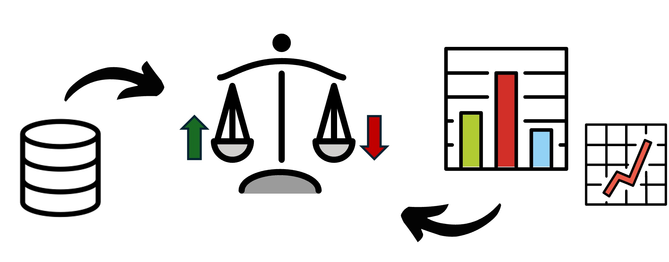
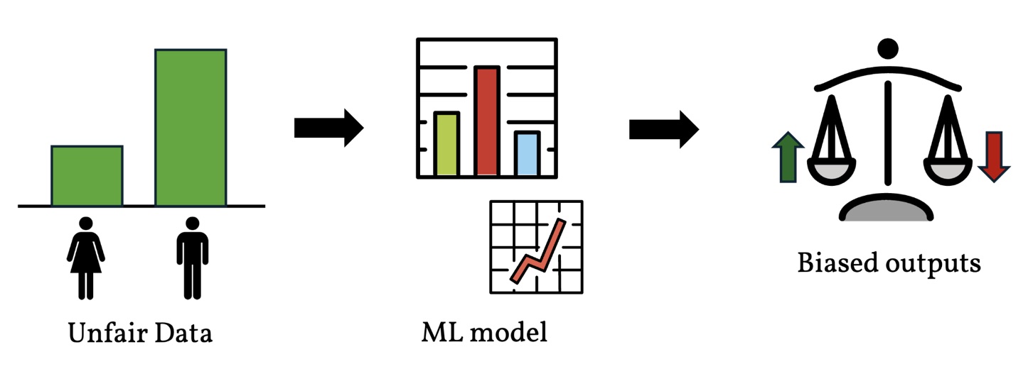An ML model trained on biased data is more likely to produce biased outputs. Scale and Charts Emojis by OpenMoji (CC BY-SA 4.0) via Streamline.

But how much bias is there, exactly? And what are ways to correct it?

Measuring bias: what makes a good yardstick?

Researchers have proposed many ways to quantify bias [Mehrabi 2021]. Most of these work by comparing the rate at which different groups receive a positive outcome (say, getting a loan). The impact ratio (IR) divides one group’s success rate by another’s: a value of 1 means equal rates, while lower or higher values suggest discrimination. The mean difference (MD) subtracts one rate from the other. The odds ratio (OR) takes a slightly different angle, comparing the odds of success between groups rather than the rates themselves. These measures are used by government agencies like the US Office of Federal Contract Compliance Programs to detect employment discrimination [Gastwirth 2021], and the well-known “four-fifths rule” flags potential discrimination when the IR falls below 0.8.

However, we found that these measures have a significant blind spot: they can give identical values for datasets that exhibit different types of (potential) discrimination. For example, we can create two datasets that have the same IR value, but for which UB=1.5% and UB=75%. In our loan example, this means IR treats both datasets the same, even though in one, women are getting nearly the expected number of loans, while in the other, they are getting only a quarter of what fairness would require.

Why does this matter? Because UB captures a very intuitive notion of discrimination: the percentage by which a group’s success rate deviates from the overall population’s rate for that outcome. For instance, if the population-wide rate of getting a loan is 24%, but only 11% of women do, UB tells us that women’s rate is roughly 55% below what we’d expect under fairness. In simple terms, 11% is about 55% less than 24%, and that is exactly what UB measures. A UB of 0 means the data is fair, and the further from 0, the more biased it is. This interpretability is precisely what allows UB to distinguish between the two datasets above, where IR could not.

Going beyond binary: intersectionality and multiple labels

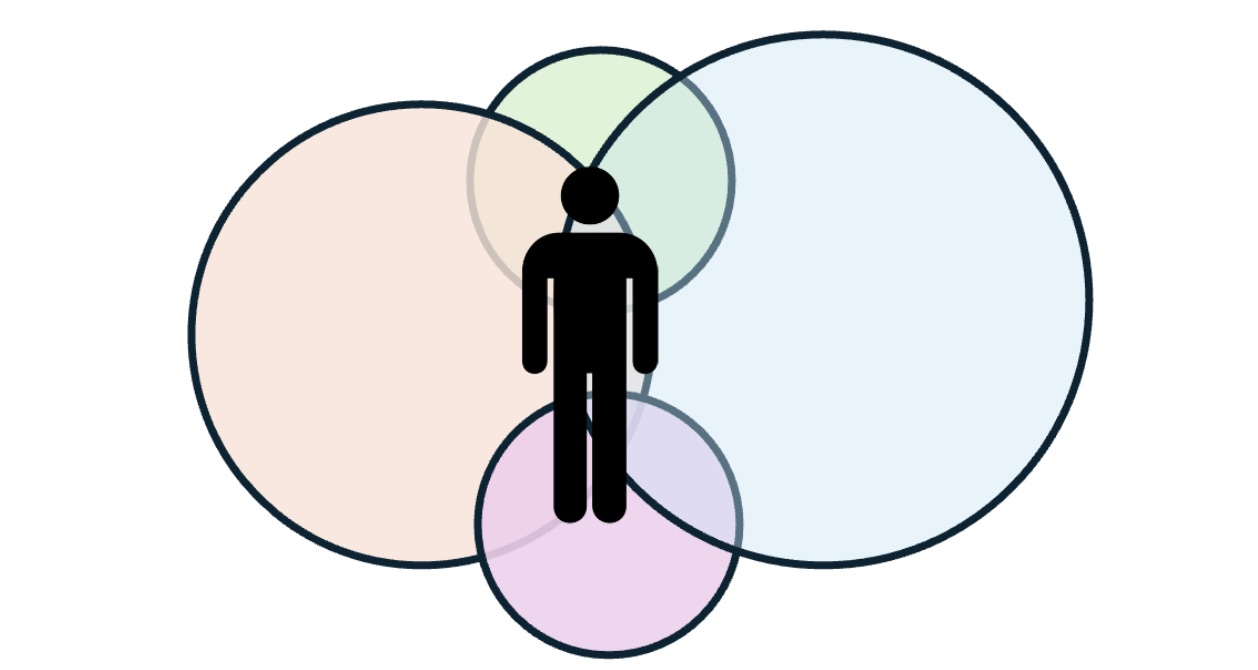Intersectionality theory establishes that fairness requires looking beyond individual attributes, since bias can hide at the intersection of gender and race.

Most prior work on bias has focused on the most simple setting: one binary sensitive attribute (e.g., male vs. female) and one binary outcome (e.g., getting a loan or not) [Wang 2022]. But real-world scenarios are more complex. The COMPAS recidivism dataset [Angwin 2016], for instance, assigns risk scores using three levels (low, medium, high) and includes both gender and race as sensitive attributes. A key insight from intersectionality research [Crenshaw 2013] is that discrimination experienced at the intersection of multiple identities (e.g., being both Black and female) can be greater than the sum of each form of discrimination individually. A dataset might appear fair when you look at gender and race separately, but reveal significant bias when you examine their intersections (both attributes at the same time) [Kearns 2019]. UB naturally extends to these more complex settings, handling multiple non-binary sensitive attributes and multi-class labels, which is essential for real-world fairness assessments but rarely supported by existing measures.

In practice, perfect statistical parity may not always be the right goal. For example, a domain expert might determine that a certain difference between groups reflects a genuine societal pattern rather than discrimination. Our framework accommodates this by allowing experts to specify their own target values for fairness, rather than always requiring zero bias. This makes the approach flexible enough to be adapted to different contexts and domains, a feature that is of key importance in ML fairness [Fleisher 2025].

Fixing the data: bias mitigation with guarantees

Detecting bias is only half the battle. We also developed a mitigation algorithm that determines exactly how many data points to add (or remove) from each demographic group to make the dataset fair. Crucially, our algorithm preserves the overall label distribution, for example in the COMPAS dataset the proportion of high, medium, and low risk scores stays the same after mitigation. This property provides a mathematical guarantee for the mitigated data to be used in the same context as the original data. Most ML algorithms and statistical methods rely on assumptions about the input distribution, so it is of key importance to preserve the representativeness of the data as much as possible for these downstream tasks.

Going back to our bank example: our framework lets the data science team explore different mitigation strategies and visualize their effects. The figure below shows a possible strategy for mitigating the bank’s dataset. Each point represents a combination of data modifications, for instance, adding records of women who get the loans (y-axis) and adding records of men who do not (x-axis). The color indicates the resulting bias: white means the data is fair, red means bias against women (as in the original dataset), and blue means bias against men. The lines mark real-world constraints, such as how much additional data is actually available. In this case, at most 3,000 records of women who get a loan and 4,500 of men who do not.

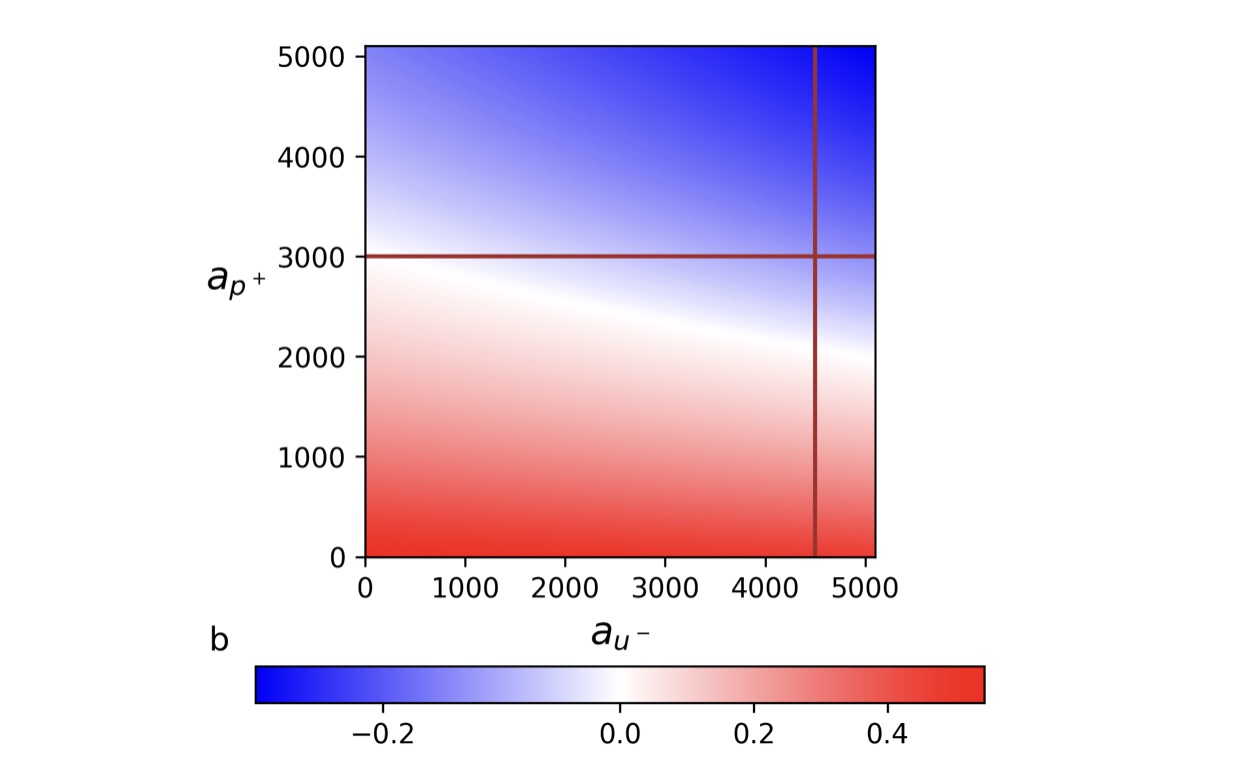A possible strategy for mitigating the bank’s dataset.

This type of visualization allows data scientists to quickly identify which combinations of modifications are feasible and how close each one gets to fairness, all before making any changes to the actual data.

Our mitigation algorithm can compute both exact and approximate solutions. The exact solution guarantees perfect fairness but may require a large number of data additions. In practice, our approximate solution achieves nearly the same fairness with far fewer additions. For example, on the COMPAS recidivism dataset, the exact solution requires over 182,000 new records, while our approximation achieves comparable results with only about 11,600, just 6.4% of the exact solution, with negligible impact on the resulting bias values.

How does bias mitigation affect ML models?

Does fairer data mean worse models? Scale Emoji by OpenMoji (CC BY-SA 4.0) via Streamline.

A natural concern when modifying data for fairness is whether the resulting models will still perform well. After all, if mitigating bias comes at a significant cost to predictive performance, practitioners may be reluctant to adopt these techniques. To investigate this, we trained six ML models on both biased and mitigated versions of three widely-used fairness benchmark datasets: Adult, Default [Default UCI], and COMPAS. The results were encouraging: In no case did bias mitigation come at a significant cost to model performance. For COMPAS with ternary labels, our mitigated data consistently outperformed the biased version across all models and metrics.

Limitations and future work

Our current approach assumes we can find or generate new data points to add to the dataset. In practice, the availability of such data depends on external sources like data lakes and domain expertise (to determine whether external data is suitable for the task). We are currently extending UB to handle coverage constraints, ensuring that all relevant demographic subgroups have sufficient representation in the mitigated data, and also exploring the trade-off between achieving perfect fairness and the resources required to get there. We also plan to investigate how our techniques can be adapted to datasets with missing values, where imputation methods may play a role.

Find out more

You can read the full paper here.

References

[Shahbazi 2023] Nima Shahbazi, Yin Lin, Abolfazl Asudeh, and HV Jagadish. 2023. Representation bias in data: A survey on identification and resolution techniques.
Comput. Surveys 55, 13s (2023), 1–39.

[Hort 2024] Hort, M.; Chen, Z.; Zhang, J. M.; Harman, M.; and Sarro, F. 2024. Bias Mitigation for Machine Learning Classifiers: A Comprehensive Survey. ACM J. Responsib. Comput., 1(2).

[Pagano 2023] Pagano, T. P.; Loureiro, R. B.; Lisboa, F. V.; Peixoto, R. M.; Guimaraes, G. A.; Cruz, G. O.; Araujo, M. M.; Santos, L. L.; Cruz, M. A.; Oliveira, E. L.; et al. 2023. Bias and unfairness in machine learning models: a systematic review on datasets, tools, fairness metrics, and identification and mitigation methods. Big data and cognitive computing, 7(1): 15.

[Mehrabi 2021] Mehrabi, N.; Morstatter, F.; Saxena, N.; Lerman, K.; and Galstyan, A. 2021. A survey on bias and fairness in machine learning. ACM computing surveys (CSUR), 54(6): 1–35.

[Gastwirth 2021] Gastwirth, J. L. 2021. A summary of the statistical aspects of the procedures for resolving potential employment discrimination recently issued by the Office of Federal Contract Compliance along with a commentary. Law, Probability and Risk, 20(2): 89–112.

[Wang 2022] Wang, A.; Ramaswamy, V. V.; and Russakovsky, O. 2022. Towards Intersectionality in Machine Learning: Including More Identities, Handling Underrepresentation, and Performing Evaluation. In Proceedings of the 2022 ACM Conference on Fairness, Accountability, and Transparency, FAccT ’22, 336–349. New York, NY, USA: Association for Computing Machinery.

[Angwin 2016] Angwin, J.; Larson, J.; Mattu, S.; and Kirchner, L. 2016. How We Analyzed the COMPAS Recidivism Algorithm.

[Crenshaw 2013] Crenshaw, K. 2013. Demarginalizing the intersection of race
and sex: A black feminist critique of antidiscrimination doctrine, feminist theory and antiracist politics. In Feminist legal theories, 23–51. Routledge.

[Kearns 2019] Kearns, M.; Neel, S.; Roth, A.; and Wu, Z. S. 2019. An Empirical
Study of Rich Subgroup Fairness for Machine Learning. In Proceedings of the Conference on Fairness, Accountability, and Transparency, FAT* ’19, 100–109. New York, NY, USA: Association for Computing Machinery.

[Fleisher 2025] Will Fleisher 2025. Algorithmic Fairness Criteria as Evidence. Ergo: An Open Access Journal of Philosophy.

[Adult UCI] Becker, B.; and Kohavi, R. 1996. Adult. UCI Machine Learning Repository.

[Default UCI] Yeh, I.-C. 2016. Default of credit card clients. UCI Machine Learning Repository.

Bruno Scarone is a Computer Science PhD candidate at Northeastern University

Bruno Scarone is a Computer Science PhD candidate at Northeastern University