
ΑΙhub.org
Strategic instrumental variable regression: recovering causal relationships from strategic responses
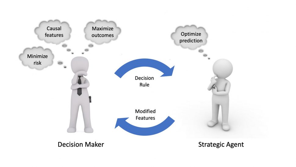
In social domains, machine learning algorithms often prompt individuals to strategically modify their observable attributes to receive more favorable predictions. As a result, the distribution the predictive model is trained on may differ from the one it operates on in deployment. While such distribution shifts, in general, hinder accurate predictions, we identify a unique opportunity associated with shifts due to strategic responses. In particular, we show that we can use strategic responses effectively to recover causal relationships between observable features and the outcomes we wish to predict. More specifically, we study a game-theoretic model in which a decision-maker deploys a sequence of models to predict an outcome of interest (e.g., college GPA) for a sequence of strategic agents (e.g., college applicants). In response, strategic agents invest efforts and modify their features for better predictions.
In such settings, unobserved confounding variables (e.g., family educational background) can influence both an agent’s observable features (e.g., high school records) and outcomes (e.g., college GPA). Because of this, standard regression methods such as ordinary least squares (OLS) generally produce biased estimators. In order to address this issue, we establish a connection between strategic responses to machine learning models and instrumental variable (IV) regression, a well-studied tool in econometrics, by observing that the sequence of deployed models can be viewed as an instrument that affects agents’ observable features, but does not directly influence their outcomes. Therefore, two-stage least squares (2SLS) regression can be used to recover the causal relationships between observable features and outcomes. Beyond causal recovery, we can use quantities learned during our 2SLS procedure to address two common optimization objectives in strategic regression: agent outcome maximization and predictive risk minimization. Finally, we empirically evaluate our methods on a semi-synthetic college admissions dataset and find that they compare favorably to OLS.
Strategic regression
When strategic agents are evaluated by algorithmic assessment tools in high-stakes situations (such as lending, education, or employment), they will modify their observable features in order to achieve a more favorable outcome. This notion is captured succinctly by Goodhart’s Law, a well-known adage by British economist Charles Goodhart, which states that
“When a measure becomes a target, it ceases to be a good measure.”
Charles Goodhart, Problems of Monetary Management: The U.K. Experience (1981)
With this idea in mind, the quickly-growing field of strategic classification/regression aims to formalize the interaction between a decision-maker, or principal, and a series of decision-subjects (often referred to as agents) as a repeated Stackelberg game (e.g., Hardt et al., 2015, Dong et al., 2018, Milli et al., 2019). At each time  , a new agent from the population interacts with the decision-maker. As a running example, consider a university (principal) which decides whether to accept or reject students (agents) on a rolling basis. The principal moves first, announcing a decision rule
  , parameterized by
  , which takes a set of observable features
  as input and produces a prediction
  as output. Having observed the decision rule , agent best responds by strategically modifying his observable features in order to receive a higher prediction score, subject to some cost for doing so. In our college admissions example, this would correspond to the university telling each student which qualities they value in an applicant (and to what extent they value them), and each applicant taking some action to improve their chances of being accepted (e.g., studying to improve their high school GPA). Most of the work in the strategic regression literature assumes the principal deploys a linear decision rule, i.e.,
  . While this assumption may limit the space of models the principal has at her disposal, it makes the agent’s best-response calculation tractable.
While the goal of each agent in the strategic regression setting is well-defined, the right objective for the principal is less obvious and is often dependent on the specific setting being considered. For example, the original work on learning under strategic responses (Hardt et al., 2015) views all feature manipulation as undesirable “gaming,” and seeks to design decision rules which minimize predictive risk under agent feature manipulation. More recent work (Kleinberg & Raghavan, 2019) makes a distinction between feature gaming and improvement, i.e., feature manipulation which leads to a positive change in the agent’s true label  . Finally, a third line of work (Shavit et al., 2020) aims to recover causal relationships between observable features and outcomes , although these methods are only applicable under settings in which all of the agent’s features that causally affect are observable to the principal. We build upon these lines of work by making the observation that the sequence of decision rules deployed by the principal can be viewed as a valid instrument, which allows us to recover causal relationships between observable features and outcomes without making the assumption that all of an agent’s features are observable. Using knowledge of these causal relationships, we then provide algorithms for agent improvement and predictive risk minimization.
Instrumental variable regression
Before getting to our method, we quickly review the basics of Instrumental Variable (IV) regression.
Imagine a situation in which a researcher is trying to estimate the causal effect that ice cream consumption has on getting sunburned. The researcher asks a group of randomly selected participants about their ice cream consumption levels, and finds that participants who consume ice cream are more likely to get sunburned in the near future. Without taking any additional variables into consideration, the researcher may come to the incorrect conclusion that eating ice cream causes one to become sunburned!
IV Regression (Angrist and Krueger, 2001) is a family of methods used to estimate causal relationships between independent and dependent variables when there exist omitted variables that affect both directly. In our ice cream example, the weather is an omitted variable that causes confounding by directly affecting both ice cream consumption levels and the likelihood of getting sunburned.

 (red line) between (e.g., ice cream consumption) and (e.g., sunburn) in the presence of an omitted variable
  (e.g., weather), by using an additional observable variable , called the instrumental variable (e.g., how hungry a person is).
We focus on two-stage least-squares (2SLS) regression (Angrist and Imbens, 1992), a kind of IV estimator. 2SLS independently estimates the relationship between an instrumental variable and the independent variables , as well as the relationship between and the dependent variable , via simple least squares regression. Formally, given  samples, 2SLS estimates the true causal relationship between and through the following procedure:
- Estimate the relationship between and as

- Estimate the relationship between and as

- Estimate the true causal relationship as

Intuitively, 2SLS allows for an unbiased estimate of by using the instrumental variable as a source of “controlled randomness.” By varying , we can observe the change in and the change in , which allows us to estimate the direct effect has on .
IV regression in the strategic learning setting
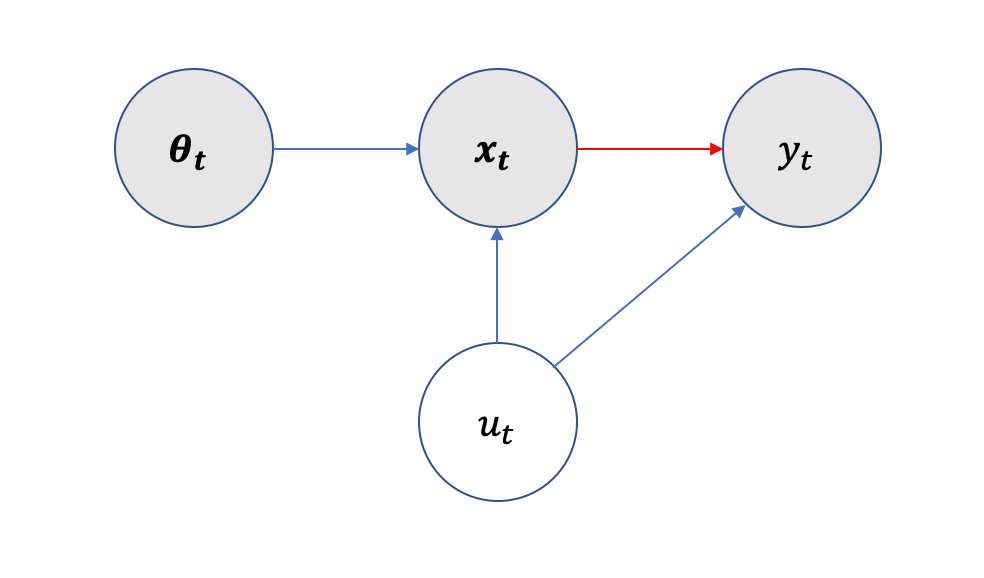
In this strategic regression setting, we make the observation that the assessment rules  are valid instruments. Therefore, we can perform IV regression to estimate the true causal parameters . There are two criteria for to be a valid instrument: (1) directly influences the observable features and only influences the outcome through , and (2) is independent from any unobservable confounding variables. In our setting, this confounding term is represented by the agent’s private type (see Figure 2 for more information). Criterion (1) is satisfied by the structure of the strategic regression setting. We aim to design a mechanism that satisfies criterion (2) by choosing assessment rule randomly, independent of the private type . As can be seen by the graphical model of our setting, the principal’s assessment rule satisfies these criteria.
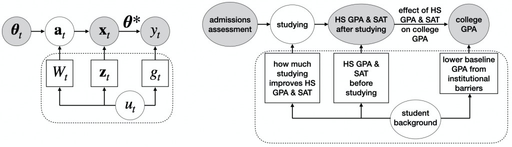 (e.g., high school GPA, SAT scores, etc.) depend on both the agent’s private type (e.g., a student’s background — whether they have family who went to college, their gender, race, ethnicity, socioeconomic status, etc.) via initial features
  (e.g. the SAT score or HS GPA student would get without studying) and effort conversion matrix
  (e.g., how much studying translates to an increase in SAT score for student ) and assessment rule via action
  (which could correspond to studying, taking an SAT prep course, etc.). An agent’s outcome (e.g. college GPA) is determined by their observable features (via causal relationship ) and type (via baseline outcome error term
  , which could be lower for students from underserved groups due to institutional barriers, discrimination, etc.).
Under mild restrictions on the agent population, if the principal plays a sequence of random assessment rules with component-wise variance at least  , our estimate
  approaches the true causal parameters at a rate of
  , with high probability. Note that while we require the principal to play random assessment rules in order to achieve our bound, we make no assumption on the mean values of the distribution are drawn from, meaning that the principal can play random perturbations of a “reasonable” assessment rule in order to achieve the desired bound.
Other principal objectives
In some settings, it may be enough for the principal to discover the true relationship between the observable features and outcome . However in other settings, the principal may wish to take a more active role. We explore two additional goals the principal may have, agent outcome maximization and predictive risk minimization, both of which are common goals in the strategic regression literature.
In the agent outcome maximization setting, the goal of the principal is to maximize the expected outcome ![\mathbb{E}[y_t]](https://aihub.org/wp-content/ql-cache/quicklatex.com-e1f788db19bc5866c0b4958ba0111c31_l3.png "Rendered by QuickLaTeX.com") of an agent from the agent population. In our running college admissions example, this would correspond to deploying an assessment rule with the goal of maximizing expected student college GPA. Note that
of an agent from the agent population. In our running college admissions example, this would correspond to deploying an assessment rule with the goal of maximizing expected student college GPA. Note that  , the assessment rule which maximizes , need not be equal to the causal parameters . Formally, we aim to find in a convex set
  of feasible assessment rules such that the induced expected agent outcome is maximized. We can formulate the problem of recovering as a convex optimization problem with a linear objective function and constraint that lie in . While this optimization has an explicit dependence on , the principal has all the information required to solve the optimization if she has already ran 2SLS to recover a sufficiently accurate estimate of the causal parameters .
On the other hand, the goal of the principal in the predictive risk minimization setting is to learn the assessment rule that minimizes ![\mathbb{E}[(y_t - \widehat{y}_t)^2]](https://aihub.org/wp-content/ql-cache/quicklatex.com-68623faae5b2ff0b9ecc08fff00ea0ba_l3.png "Rendered by QuickLaTeX.com") , the expected squared difference between an agent’s true outcome and the outcome predicted by the principal. Similar to the agent outcome maximization setting, the principal will be able to calculate the gradient of after having recovered a sufficiently accurate estimate of . Due to the dependence of and on the assessment rule deployed by the principal, the predictive risk function will be nonconvex in general, and can have several extrema which are not global minima, even in the case of just one observable feature. Because of this, natural learning dynamics like online gradient descent will generally only converge to local minima of the predictive risk function.
, the expected squared difference between an agent’s true outcome and the outcome predicted by the principal. Similar to the agent outcome maximization setting, the principal will be able to calculate the gradient of after having recovered a sufficiently accurate estimate of . Due to the dependence of and on the assessment rule deployed by the principal, the predictive risk function will be nonconvex in general, and can have several extrema which are not global minima, even in the case of just one observable feature. Because of this, natural learning dynamics like online gradient descent will generally only converge to local minima of the predictive risk function.
Experiments
We empirically evaluate our model on a semi-synthetic dataset based on our running university admissions example, and compare our 2SLS-based method against OLS, which directly regresses observed outcomes  on observable features
  . We constructed our semi-synthetic dataset by modifying the SATGPA dataset, a publicly available dataset which contains statistics on 1000 college students. We use high school (HS) grades, as measured by grade point average (GPA) and SAT score as observable features, and college GPA as the outcome. Using OLS, we find that the effect of [SAT, HS GPA] on college GPA in this dataset is
 ![\boldsymbol{\theta}^*= [0.0015, 0.5895]](https://aihub.org/wp-content/ql-cache/quicklatex.com-145c03a69443e774c0e208902f9036d1_l3.png "Rendered by QuickLaTeX.com") . We then construct synthetic data that is based on this original data, yet incorporates confounding factors. For simplicity, we let the true effect
. We then construct synthetic data that is based on this original data, yet incorporates confounding factors. For simplicity, we let the true effect ![\boldsymbol{\theta}^* = [0, 0.5]](https://aihub.org/wp-content/ql-cache/quicklatex.com-489c23cf3c99e92bddeb63dd73fa0c2b_l3.png "Rendered by QuickLaTeX.com") . That is, we assume HS GPA affects college GPA, but SAT score does not. We consider two private types of applicant backgrounds: disadvantaged and advantaged. Disadvantaged applicants have lower initial HS GPA and SAT (
. That is, we assume HS GPA affects college GPA, but SAT score does not. We consider two private types of applicant backgrounds: disadvantaged and advantaged. Disadvantaged applicants have lower initial HS GPA and SAT ( ), lower baseline college GPA (
 ), and need more effort to improve their observable features (
 ). Each applicant’s initial features are randomly drawn from one of two distributions, depending on background. Please note that our semi-synthetic dataset is for illustrative purposes only; we are not making any claims about the extent to which SAT, GPA, etc. should be used in college admissions decisions.
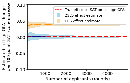
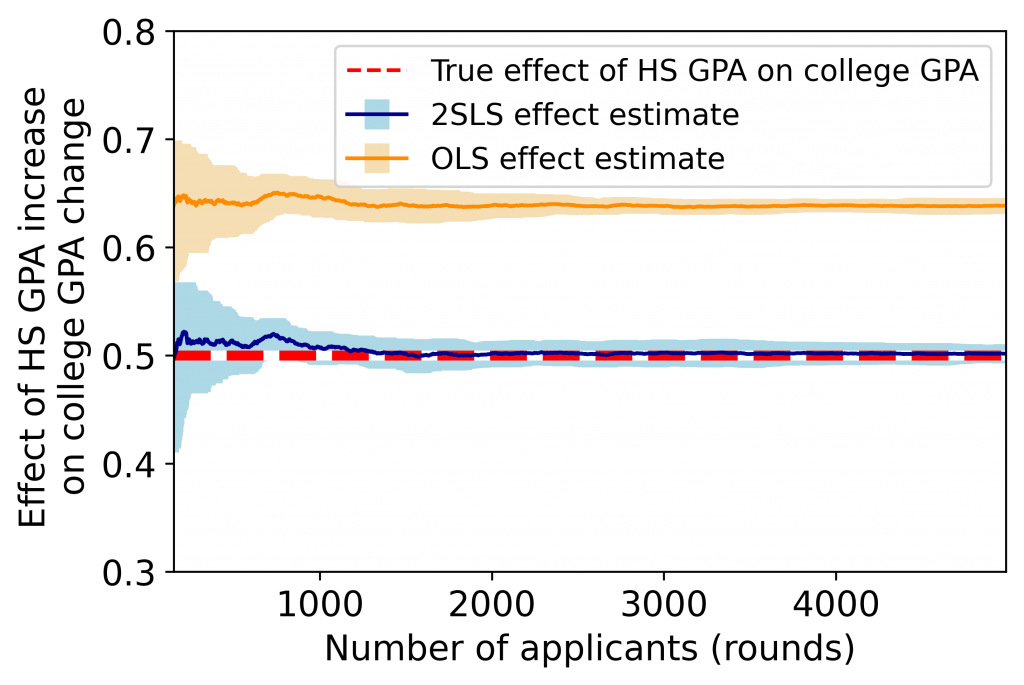
As can be seen by the above figures, our 2SLS method converges to the true effect parameters, whereas OLS has a constant bias. Notably, OLS mistakenly predicts that, on average, a 100 point increase in SAT score leads to about a 0.05 point increase in college GPA, even though the two are not causally related in our synthetic dataset. Moreover, we note that the estimation error of 2SLS empirically decreases at the predicted rate of  .
.
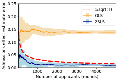
 (in orange) and 2SLS estimate error
  (in blue) over 5000 rounds. Results are averaged over 10 runs. Error bars (in lighter colors) represent one standard deviation.
Conclusion and discussion
In this work, we established the possibility of recovering the causal relationship between observable attributes and the outcome of interest in settings where a decision-maker utilizes a series of linear assessment rules to evaluate strategic individuals. Our key observation was that in such settings, assessment rules serve as valid instruments (because they causally impact observable attributes but do not directly cause changes in the outcome). This observation enables us to present a 2SLS method to correct for confounding bias in causal estimates. Armed with accurate estimates of the causal parameters, we additionally provide algorithms for two common principal objectives:agent outcome maximization and predictive risk minimization. Finally, we empirically evaluate our methods on a semi-synthetic college admissions dataset and find that our methods outperform standard OLS regression.
Our work offers a practical approach for inferring causal relationships while employing reasonably accurate decision-making models. Knowledge of causal relationships in social domains can improve the robustness of ML-based decision-making systems to gaming and manipulation, facilitate auditing these systems for compliance with policy goals such as fairness, and allow planning for better societal outcomes. While our work offers an initial step toward extracting causal knowledge from a series of automated decisions, we rely on several simplifying assumptions, all of which mark essential directions for future work. For instance, we assumed all assessment rules and the underlying causal model are linear. This assumption allowed us to utilize linear IV methods. Extending our work to non-linear assessment rules and IV methods is necessary for the applicability of our method to real-world automated decision-making. Another critical assumption we made was the agent’s full knowledge of the assessment rule and their rational response to it subject to a quadratic effort cost. While these are standard assumptions in economic modeling, they need to be empirically verified in the particular decision-making context at hand before our method’s outputs can be viewed as reliable estimates of causal relationships.
For details about our method, mathematical derivations, full experimental results, etc., see our paper here.
This article was initially published on the ML@CMU blog and appears here with the authors’ permission.
tags: deep dive

AUAI is supported by: