
ΑΙhub.org
An experimental design perspective on model-based reinforcement learning
By Viraj Mehta and Willie Neiswanger
Reinforcement learning (RL) has achieved astonishing successes in domains where the environment is easy to simulate. For example, in games like Go or those in the Atari library, agents can play millions of games in the course of days to explore the environment and find superhuman policies [1]. However, transfer of these advances to broader real-world applications is challenging because the cost of exploration in many important domains is high. For example, while RL-based solutions for controlling plasmas in the nuclear fusion power generation are promising, there is only one operating tokamak in the United States and its resources are in excessive demand. Even the most data-efficient RL algorithms typically take thousands of samples to solve even moderately complex problems [2, 3], which is infeasible in plasma control and many other applications.
In contrast to conventional machine learning settings where the data is given to the decision maker, an RL agent can choose data to learn from. A natural idea for reducing data requirements is to choose data wisely such that a smaller amount of data is sufficient to perform well on a task. In this post, we describe a practical implementation of this idea. Specifically, we offer an answer to the following question: “If we were to collect one additional datapoint from anywhere in the state-action space to best improve our solution to the task, which one would it be?”. This question is related to a more fundamental idea in the design of intelligent agents with limited resources: such agents should be able to understand what information about the world is the most useful to help them accomplish their task. We see this work as a small step towards this bigger goal.
In our recent ICLR paper, “An Experimental Design Perspective on Model-Based Reinforcement Learning“, we derive an acquisition function that guides an agent in choosing data for the most successful learning. In doing this, we draw a connection between model-based reinforcement learning and Bayesian optimal experimental design (BOED) and evaluate data prospectively in the context of the task reward function and the current uncertainty about the dynamics. Our approach can be efficiently implemented under a conventional assumption of a Gaussian Process (GP) prior on the dynamics function. Typically in BOED, acquisition functions are used to sequentially design experiments that are maximally informative about some quantity of interest by repeatedly choosing the maximizer, running the experiment, and recomputing the acquisition function with the new data. Generalizing this procedure, we propose a simple algorithm that is able to solve a wide variety of control tasks, often using orders of magnitude less data than competitor methods to reach similar asymptotic performance.
Preliminaries
In this work, we consider a RL agent that operates in an environment with unknown dynamics. This is a general RL model for decision-making problems in which the agent starts without any knowledge on how their actions impact the world. The agent then can query different state-action pairs to explore the environment and find a behavior policy that results in the best reward. For example, in the plasma control task, the states are various physical configurations of the plasma and possible actions include injecting power and changing the current. The agent does not have prior knowledge on how its actions impact the conditions of the plasma. Thus, it needs to quickly explore the space to ensure efficient and safe operation of the physical system—a requirement captured in the corresponding reward function.
Given that each observation of a state-action pair is costly, an agent needs to query as few state-action pairs as possible and in this work we develop an algorithm that informs the agent about which queries to make.
We operate under a setting we call transition query reinforcement learning (TQRL). In this setting, an agent can can sequentially query the dynamics at arbitrary states and actions to learn a good policy, essentially teleporting between states as it wishes. Traditionally, in the rollout setting, agents must simply choose actions and execute entire episodes to collect data. TQRL therefore is a slightly more informative form of access to the real environment.
Precise Definition of the Setup
More precisely: we address finite-horizon discrete time Markov Decision Processes (MDPs), which consist of a tuple  where:
 is the state space
 is the action space
 (dynamics) is the stochastic transition function that maps (state, action) pairs
  to a probability distribution over states
  is a reward function
 is a start distribution over states
 is an integer-valued horizon, that is, the number of steps the agent will perform in the environment
We assume that all of these parameters are known besides dynamics . The key quantity that defines the behaviour of the agent is its policy  that tells the agent what action to take in a given state. Thus, the overall goal of the agent is to find a policy that maximizes the cumulative reward over the agent’s trajectory
  followed by the agent. Formally, a trajectory is simply a sequence of (state, action) pairs
 ![\tau = [s_0, a_0, \dots, a_{H -1}, s_H]](https://aihub.org/wp-content/ql-cache/quicklatex.com-ae105c8081bdc61ab2c18c8290650888_l3.png "Rendered by QuickLaTeX.com") , where
, where  is an action taken by the agent at step
  and
and  is a state in which agent was at time . Denoting the cumulative reward over trajectory
  as
as  , the agent needs to solve the following optimization problem:
![\[\max_\pi \mathbb{E}_{\tau \sim p(\tau\mid \pi, T)}\left[R(\tau)\right].\]](https://aihub.org/wp-content/ql-cache/quicklatex.com-b435d0c41bdcb7af5cc7a8f0973df5cd_l3.png "Rendered by QuickLaTeX.com")
We call an optimal policy for a given dynamics as  . As we know the other parts of the MDP, to solve the optimization problem, we need to learn a model for the transition function
  .
.
Main Idea
Inspired by BOED and Bayesian algorithm execution (BAX) [11], we use ideas from information theory to motivate our method to effectively choose data points. Our goal is to sequentially choose queries  such that our agent quickly finds a good policy. We observe that to perform the task successfully, we do not need to approximate the optimal policy
  everywhere in the state space. Indeed, there could be regions of the state space that are unlikely to be visited by the optimal policy. Thus, we only need to approximate the optimal policy in the regions of the state space that are visited by the optimal policy.
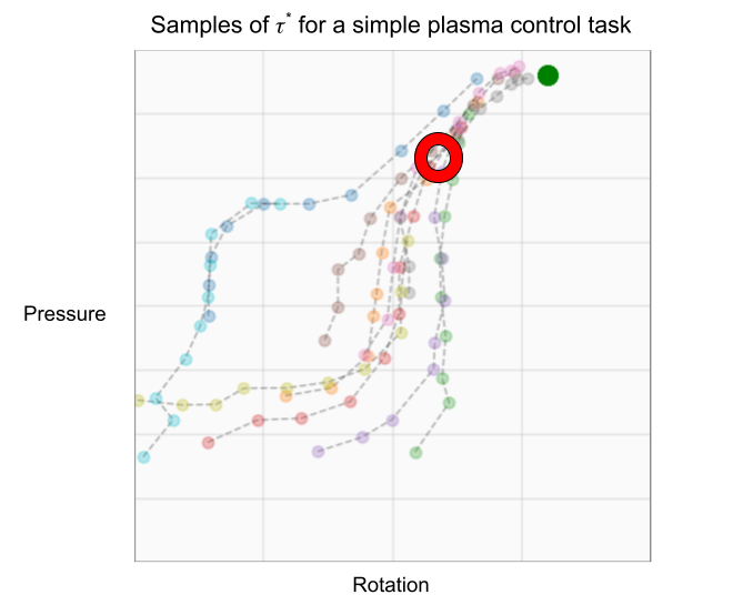
Therefore, we choose to learn about  —the optimal trajectory governed by the optimal policy . This objective only requires data about the areas we believe will visit as it solves the task, so intuitively we should not “waste” samples on irrelevant regions in the state-action space. In plasma control, this idea might look like designing experiments in certain areas of the state and action space that will teach us the most about controlling plasma in the target regimes we need to maintain fusion.
We thus define our acquisition function to be the expected information gain about from sampling a point  given a dataset
  :
:
![\[EIG_{\tau^*}(s, a) = \mathbb{H}[\tau^* \mid D] - \mathbb{E}_{s'\sim T(s, a)}\left[\mathbb{H}b[\tau^*\mid D\cup \{(s, a, s')\}]\right].\]](https://aihub.org/wp-content/ql-cache/quicklatex.com-2a527da3282d70931096231deacbc705_l3.png "Rendered by QuickLaTeX.com")
Intuitively, this quantity measures how much the additional data is expected to reduce the uncertainty (here given by Shannon entropy, denoted  ) about the optimal trajectory.
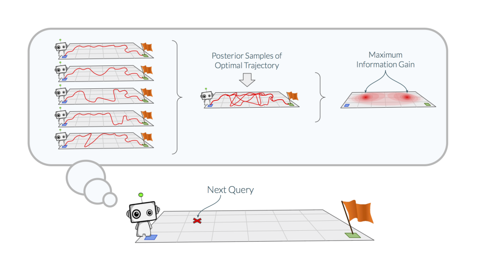
At a high level, following methods related to the InfoBAX algorithm [11], we can approximate this acquisition function by a three-step procedure:
- First, we sample many possible dynamics functions from our posterior (e.g., functions that describe plasma evolution).
- Second, we find optimal trajectories on each of the sampled dynamics functions without taking new data from the environment, as we can simulate controls on these dynamics.
- Third, we compute predictive entropies of our model at and of our model with additional data taken from each optimal trajectory. We can then subtract the trajectory-conditioned entropy from the original entropy.
This final step allows us to estimate the mutual information between  and , which is precisely the quantity we want. We give a more precise description of this below.
Computing  via posterior function sampling
More formally: as is a high-dimensional object that implicitly assumes access to an optimal decision making policy, it is not obvious that the entropies involved in computing it will be easy to estimate. However, by making two additional assumptions and leveraging properties of mutual information, we can derive a practical method for estimating . In particular, we need to assume that:
- The dynamics are drawn from a GP prior
 , a fairly mild assumption since GPs are universal approximators [10].
  for an MDP with known rewards and transition function , i.e., that a model-predictive control (MPC) policy using known dynamics will be close to optimal on those dynamics. This is not true in all settings and we investigate how crucial this assumption is to the performance of the algorithm in our experiments section.
We know from information theory that
 where
where  refers to the mutual information. This expression is much easier to deal with, given a GP. We can use the fact that given a GP prior the marginal posterior at any point in the domain is a Gaussian in closed form, to exactly compute the left term
 ![\mathbb{H}[T(s, a)\mid D]](https://aihub.org/wp-content/ql-cache/quicklatex.com-2b6905fb9e69676e6a8c193cc790f4c8_l3.png "Rendered by QuickLaTeX.com") . We compute the right term
. We compute the right term ![\mathbb{E}_{\tau^\sim P(\tau^ \mid D)}\left[\mathbb{H}[T(s, a)\mid D\cup \tau^*]\right]](https://aihub.org/wp-content/ql-cache/quicklatex.com-8399d2093dbfac418207fa79cbd06e04_l3.png "Rendered by QuickLaTeX.com") via a Monte Carlo approximation, sampling
via a Monte Carlo approximation, sampling  (doable efficiently due to [6]) and then sampling trajectories
  by executing MPC using
  as both the dynamics model used for planning and the dynamics function of the MDP used to sample transitions in . As is a sequence of state-action transitions, it is essentially made of more data for our estimate of the transition model. So it is straightforward to compute the model posterior
  (which again must be Gaussian) and read off the entropy of the prediction. The full Monte Carlo estimator is
![\[EIG_{\tau^*}(s, a) \approx \mathbb{H}[T(s, a)\mid D] - \frac{1}{n}\sum_{i \in [n]}\mathbb{H}[T(s, a)\mid D\cup \tau_i]\]](https://aihub.org/wp-content/ql-cache/quicklatex.com-ae51efec7ddea7b3e653d97d3b8b79b5_l3.png "Rendered by QuickLaTeX.com")
for  sampled as described above.
In summary, we can estimate our acquisition function via the following procedure, which is subject to the two assumptions listed above:
- Sample many functions

- Sample trajectories
 by executing the MPC policy
  on the dynamics
  .
. - Compute the entropies and
![\mathbb{H}[T(s, a)\mid D\cup \tau_i]](https://aihub.org/wp-content/ql-cache/quicklatex.com-ac4eeb4ad831193da0e379def820bcc1_l3.png "Rendered by QuickLaTeX.com") , for all , using standard GP techniques.
, for all , using standard GP techniques. - Compute the acquisition function using our Monte Carlo estimator.
Inspired by the main ideas of BOED and active learning, we give a simple greedy procedure which we call BARL (Bayesian Active Reinforcement Learning) for using our acquisition function to acquire data given some initial dataset:
- Compute
 given the dataset for a large random set of state-action pairs. Samples of can be reused between these points.
 - Sample
 for the
  that was found to maximize the acquisition function and add (s, a, s’) to the dataset.
 - Repeat steps 1-2 until the query budget is exhausted. The evaluation policy is simply MPC on the GP posterior mean.
Does BARL reduce the data requirements of RL?
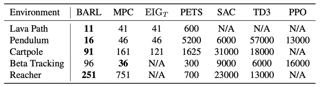
We evaluate BARL on the TQRL setting in 5 environments which span a variety of reward function types, dimensionalities, and amounts of required data. In this evaluation, we estimate the minimum amount of data an algorithm needs to learn a controller. The evaluation environments include the standard underactuated pendulum swing-up task, a cartpole swing-up task, the standard 2-DOF reacher task, a navigation problem where the agent must find a path across pools of lava, and a simulated nuclear fusion control problem where the agent is tasked with modulating the power injected into the plasma to achieve a target pressure.
To assess the performance of BARL in solving MDPs quickly, we assembled a group of reinforcement learning algorithms that represent the state of the art in solving continuous MDPs. We compare against model-based algorithms PILCO [7], PETS [2], model-predictive control with a GP (MPC), and uncertainty sampling with a GP ( ), as well as model-free algorithms SAC [3], TD3 [8], and PPO [9]. Besides the uncertainty sampling (which operates in the TQRL setting and is directly comparable to BARL), these methods rely on the rollout setting for RL and are somewhat disadvantaged relative to BARL.
BARL clearly outperforms each of the comparison methods in nearly every problem in data efficiency. We see that simpler methods like and MPC perform well on lower-dimensional problems like Lava Path, Pendulum, and Beta Tracking, but struggle with the higher-dimensional Reacher Problem. Model-free methods like SAC, TD3, and PPO are notably sample-hungry.
After further investigation, we also find that models that used data chosen by BARL are more accurate on the datapoints required to solve the problem and less accurate on a randomly chosen test set of points than models using data chosen via . This implies that BARL is choosing the ‘right data’. Since the same model is used in both of these methods, there will inevitably be areas of the input space where each of the methods performs better than the other. BARL performs better on the areas that are needed to solve the problem.
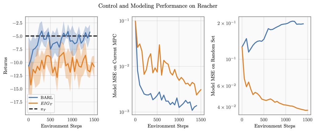 on three criteria. In the left chart, we plot control performance as queries are made.
  is the performance of MPC with a perfect model. In the middle, we plot modeling errors for BARL vs on the points where the model is queried in order to plan actions. On the right, we plot modeling errors on a uniform test set. BARL models the dynamics well on the points required to plan the optimal actions (middle) while not learning the dynamics well in general (right). This focus on choosing relevant datapoints allows BARL to solve the task quickly (left).
Conclusion
We believe is an important first step towards agents that think proactively about the data that they will acquire in the future. Though we are encouraged by the strong performance we have seen so far, there is substantial future work to be done. In particular, we are currently working to extend BARL to the rollout setting by planning actions that will lead to maximum information in the future. We also aim to solve problems of scaling these ideas to the high-dimensional state and action spaces that are necessary for many real-world problems.
References
[1] Mastering the game of Go with deep neural networks and tree search, Silver et al, Nature 2016
[2] Deep Reinforcement Learning in a Handful of Trials using Probabilistic Dynamics Models, Chua et al, Neurips 2018
[3] Soft Actor-Critic: Off-Policy Maximum Entropy Deep Reinforcement Learning with a Stochastic Actor, Haarnoja et al, ICML 2018
[4] Cross-Entropy Randomized Motion Planning, Kobilarov et al, RSS 2008
[5] Sample-efficient Cross-Entropy Method for Real-time Planning, Pinneri et al, CoRL 2020
[6] Efficiently Sampling Functions from Gaussian Process Posteriors, Wilson et al, ICML 2020
[7] PILCO: A Model-Based and Data-Efficient Approach to Policy Search, Deisenroth & Rasmussen, ICML 2011
[8] Addressing Function Approximation Error in Actor-Critic Methods, Fujimoto et al, ICML 2018
[9] Proximal Policy Optimization Algorithms, Schulman et al, 2017
[10] Universal Kernels, Micchelli et al, JMLR 2006
[11] Bayesian Algorithm Execution: Estimating Computable Properties of Black-box Functions Using Mutual Information, Neiswanger et al, ICML 2021
This article was initially published on the ML@CMU blog and appears here with the authors’ permission.
tags: deep dive

AUAI is supported by: