Deep attentive variational inference

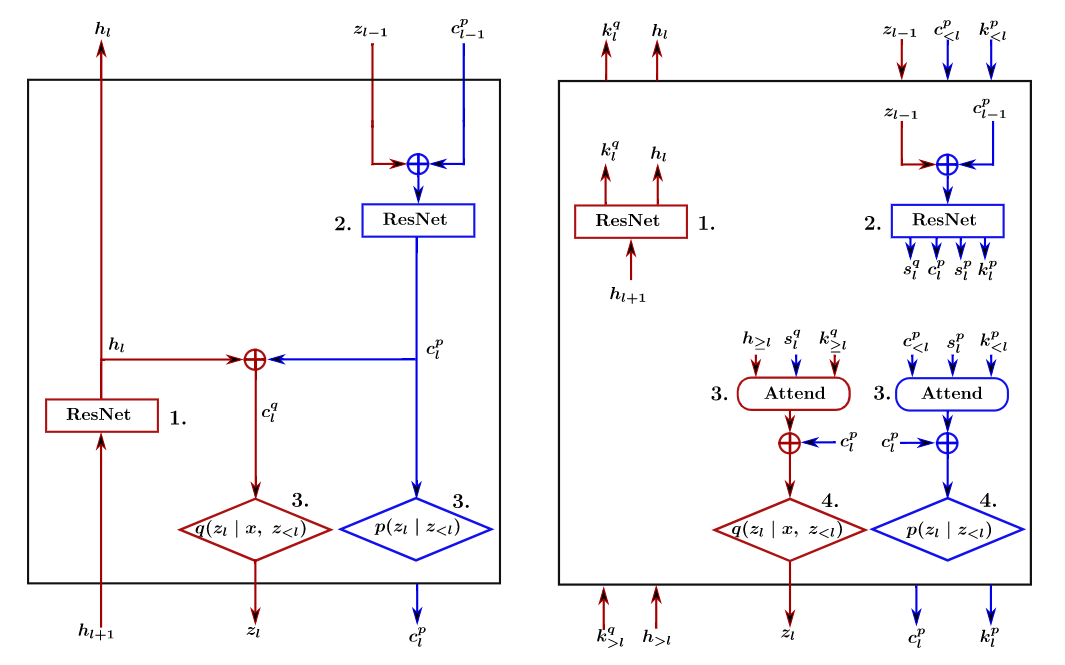
Figure 1: Overview of a local variational layer (left) and an attentive variational layer (right) proposed in this post. Attention blocks in the variational layer are responsible for capturing long-range statistical dependencies in the latent space of the hierarchy.

By Ifigeneia Apostolopoulou

Generative models are a class of machine learning models that are able to generate novel data samples such as fictional celebrity faces, digital artwork, and scenic images. Currently, the most powerful generative models are deep probabilistic models. This class of models uses deep neural networks to express statistical hypotheses about the data generation process, and combine them with latent variable models to augment the set of observed data with latent (unobserved) information in order to better characterize the procedure that generates the data of interest.

In spite of these successful results, deep generative modeling remains one of the most complex and expensive tasks in AI. Recent models rely on increased architectural depth to improve performance. However, as we show in our paper [1], the predictive gains diminish as depth increases. Keeping a Green-AI perspective in mind when designing such models could lead to their wider adoption in describing large-scale, complex phenomena.

A quick review of Deep Variational AutoEncoders

Latent variable models augment the set of observed variables with auxiliary latent variables. They are characterized by a posterior distribution over the latent variables, one which is generally intractable and typically approximated by closed-form alternatives. Moreover, they provide an explicit parametric characterization of the joint distribution over the expanded random variable space. The generative and the inference portions of such a model are jointly trained. The Variational AutoEncoder (VAE) belongs to this model category. Figure 2 provides an overview of a VAE.

VAEs are trained by maximizing the Evidence Lower BOund (ELBO) which is a tractable, lower bound of the marginal log-likelihood:

The most powerful VAEs introduce large latent spaces that are organized in blocks such that , with each block being generated by a layer in a hierarchy. Figure 3 illustrates a typical architecture of a hierarchical VAE. Most state-of-the-art VAEs correspond to a fully connected probabilistic graphical model. More formally, the prior distribution follows the factorization:

   

In words, depends on all previous latent factors . Similarly, the posterior distribution is given by:

   

The long-range conditional dependencies are implicitly enforced via deterministic features that are mixed with the latent variables and are propagated through the hierarchy. Concretely, each layer is responsible for providing the next layer with a latent sample along with context information :

   

In a convolutional VAE, is a non-linear transformation implemented by ResNet blocks as shown in Figure 1. The operator combines two branches in the network. Due to its recursive definition, is a function of .

Deep Variational AutoEncoders are “overthinking”

Recent models such as NVAE [2] rely on increased depth to improve performance and deliver results comparable to that of purely generative, autoregressive models while permitting fast sampling through a single network evaluation. However, as we show in our paper and Table 1, the predictive gains diminish as depth increases. After some point, even if we double the number of layers, we can only realize a slight increase in the marginal likelihood.

Depth	bits/ dim
2	3.5	–
4	3.26	-6.8
8	3.06	-6.1
16	2.96	-3.2
30	2.91	-1.7

We argue that this may be because the effect of the latent variables of earlier layers diminishes as the context feature traverses the hierarchy and is updated with latent information from subsequent layers. In turn, this means that in practice the network may no longer respect the factorization of the variational distributions of Equations (1) and (2), leading to sub-optimal performance. Formally, large portions of early blocks collapse to their prior counterparts, and therefore, they no longer contribute to inference.

This phenomenon can be attributed to the local connectivity of the layers in the hierarchy, as shown in Figure 4.a. In fact, a layer is directly connected only with the adjacent layers in a deep VAE, limiting long-range conditional dependencies between and as depth increases.

The flexibility of the prior and the posterior can be improved by designing more informative representations for the conditioning factors of the conditional distributions and . This can be accomplished by designing a hierarchy of densely connected stochastic layers that dynamically learn to attend to latent and observed information most critical to inference. A high-level description of this idea is illustrated in Figure 4.b.

In the following sections, we describe the technical tool that allows our model to realize the strong couplings presented in Figure 4.b.

Problem: Handling long sequences of large 3D tensors

In deep convolutional architectures, we usually need to handle long sequences of large 3D context tensors. A typical sequence is shown in Figure 5. Constructing effectively strong couplings between current and previous layers in a deep architecture can be formulated as:

Problem definition: Given a sequence of contexts with , we need to construct a single context that summarizes information in that is most critical to the task.

In our framework, the task of interest is the construction of posterior and prior beliefs. Equivalently, contexts and represent the conditioning factor of the posterior and prior distribution of layer .

There are two ways to view a long sequence of large -dimensional contexts:

• Inter-Layer couplings: As independent pixel sequences of dimensional features of length . One such sequence is highlighted in Figure 5.
• Intra-Layer couplings: As independent pixel sequences of dimensional features of length .

This observation leads to a factorized attention scheme that identifies important long-range, inter-layer, and intra-layer dependencies separately. Such decomposition of large and long pixel sequences leads to significantly less compute.

Inter-Layer couplings: Depth-wise Attention

The network relies on a depth-wise attention scheme to discover inter-layer dependencies. The task is characterized by a query feature . During this phase, the pixel sequences correspond to instances of a pixel at the previous layers in the architecture. They are processed concurrently and independently from the rest. The contexts are represented by key features of a lower dimension. The final context is computed as a weighted sum of the contexts according to an attention distribution. The mechanism is explained in Figure 6.

The layers in the variational hierarchy are augmented with two depth-wise attention blocks for constructing the context of the prior and posterior distribution. Figure 1 displays the computational block of an attentive variational layer. As shown in Figure 6, each layer also needs to emit attention-relevant features: the keys and queries , along with the contexts . Equation (3) is revised for the attention-driven path in the decoder such that the context, its key, and the query are jointly learned:

   

A formal description along with normalization schemes are provided in our paper.

Intra-Layer couplings: Non-local blocks

Intra-layer dependencies can be leveraged by interleaving non-local blocks [3] with the convolutions in the ResNet blocks of the architecture, also shown in Figure 1.

Experiments

We evaluate Attentive VAEs on several public benchmark datasets of both binary and natural images. In Table 2, we show performance and training time of state-of-the-art, deep VAEs on CIFAR-10. CIFAR-10 is a 32×32 natural images dataset. Attentive VAEs achieve state-of-the-art likelihoods compared to other deep VAEs. More importantly, they do so with significantly fewer layers. Fewer layers mean decreased training and sampling time.

Model	Layers	Training Time (GPU hours)	(bits/dim)
Attentive VAE, 400 epochs [1]	16	272	2.82
Attentive VAE, 500 epochs [1]	16	336	2.81
Attentive VAE, 900 epochs [1]	16	608	2.79
NVAE [2]	30	440	2.91
Very Deep VAE [4]	45	288	2.87

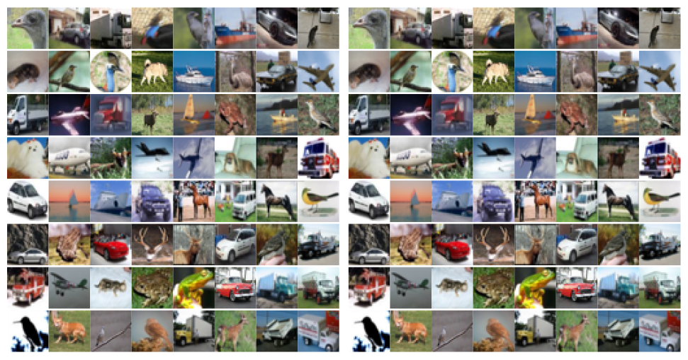
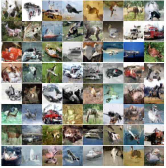
In Figures 8 and 9, we show reconstructed and novel images generated by attentive VAE. Attentive VAE achieves high-quality and diverse novel samples without restricting the prior to high-probability areas as is done in [2].

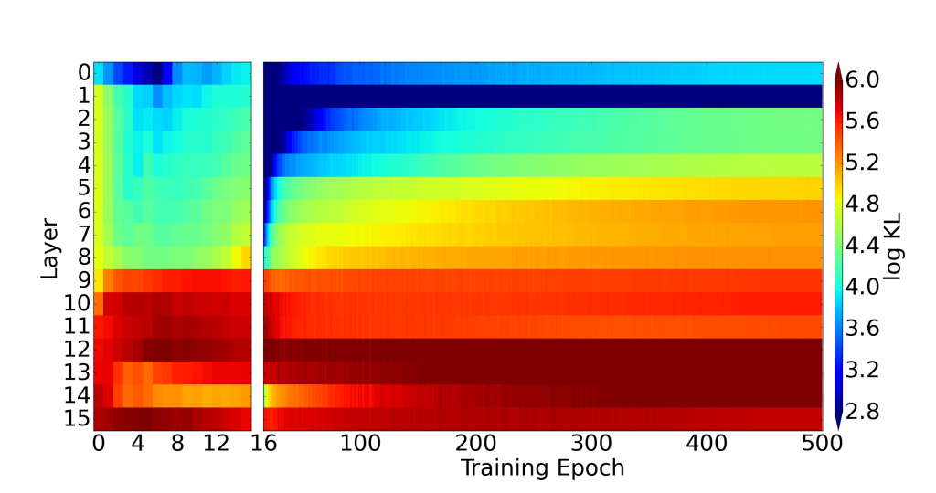
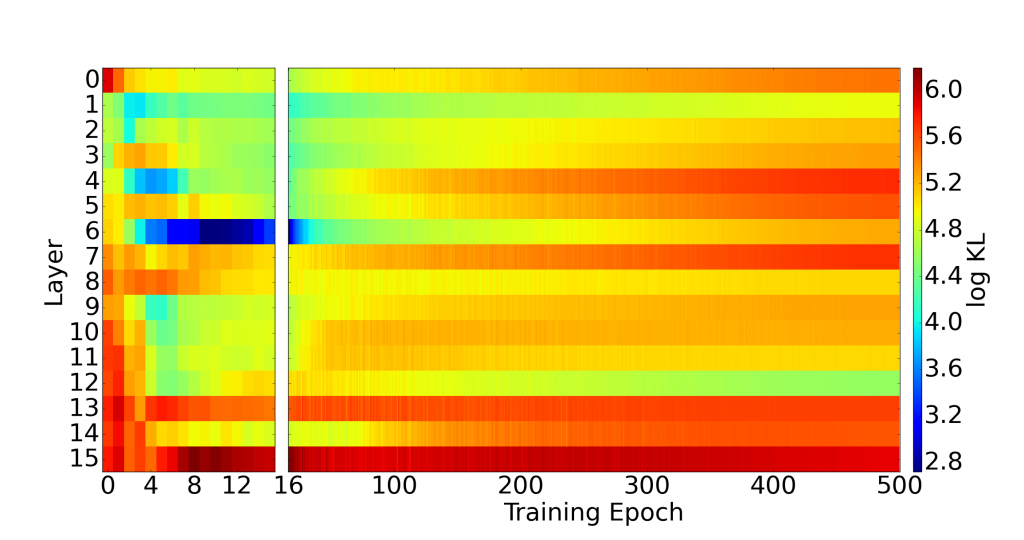
The reason behind this improvement is that the attention-driven, long-range connections between layers lead to better utilization of the latent space. In Figure 7, we visualize the KL divergence per layer during training. As we see in (b), the KL penalty is evenly distributed among layers. In contrast, as shown in (a), the upper layers in a local, deep VAE are significantly less active. This confirms our hypothesis that the fully-connected factorizations of Equations (1) and (2) may not be supported by local models. In contrast, an attentive VAE dynamically prioritizes statistical dependencies between latent variables most critical to inference.

Finally, attention-guided VAEs close the gap in the performance between variational models and expensive, autoregressive models. Comprehensive comparisons, quantitative and qualitative results are provided in our paper.

Conclusion

The expressivity of current deep probabilistic models can be improved by selectively prioritizing statistical dependencies between latent variables that are potentially distant from each other. Attention mechanisms can be leveraged to build more expressive variational distributions in deep probabilistic models by explicitly modeling both nearby and distant interactions in the latent space. Attentive inference reduces computational footprint by alleviating the need for deep hierarchies.

Acknowledgments

A special word of thanks is due to Christos Louizos for helpful pointers to prior works on VAEs, Katerina Fragkiadaki for helpful discussions on generative models and attention mechanisms for computer vision tasks, Andrej Risteski for insightful conversations on approximate inference, and Jeremy Cohen for his remarks on a late draft of this work. Moreover, we are very grateful to Radium Cloud for granting us access to computing infrastructure that enabled us to scale up our experiments. We also thank the International Society for Bayesian Analysis (ISBA) for the travel grant and the invitation to present our work as a contributed talk at the 2022 ISBA World Meeting. This material is based upon work supported by the Defense Advanced Research Projects Agency under award number FA8750-17-2-0130, and by the National Science Foundation under grant number 2038612. Moreover, the first author acknowledges support from the Alexander Onassis Foundation and from A. G. Leventis Foundation. The second author is supported by the National Science Foundation Graduate Research Fellowship Program under Grant No. DGE1745016 and DGE2140739.

DISCLAIMER: All opinions expressed in this post are those of the author and do not represent the views of CMU.

References

[1] Apostolopoulou I, Char I, Rosenfeld E, Dubrawski A. Deep Attentive Variational Inference. InInternational Conference on Learning Representations 2021 Sep 29.

[2] Vahdat A, Kautz J. Nvae: A deep hierarchical variational autoencoder. Advances in Neural Information Processing Systems. 2020;33:19667-79.

[3] Wang X, Girshick R, Gupta A, He K. Non-local neural networks. InProceedings of the IEEE conference on computer vision and pattern recognition 2018 (pp. 7794-7803).

[4] Child R. Very deep vaes generalize autoregressive models and can outperform them on images. arXiv preprint arXiv:2011.10650. 2020 Nov 20.

Want to learn more?

Check out:

• Our paper
• Our poster
• Our presentation
• Our source code

This article was initially published on the ML@CMU blog and appears here with the authors’ permission.

ML@CMU

ML@CMU