Causal confounds in sequential decision making

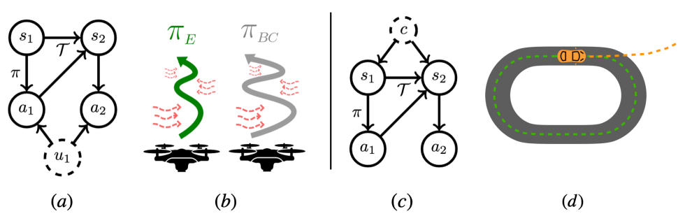
A standard assumption in sequential decision making is that we observe everything required to make good decisions. In practice however, this isn’t always the case. We discuss two specific examples (temporally correlated noise (a) and unobserved contexts (c)) that have stymied the use of IL/RL algorithms (in autonomous helicopters (b) and self-driving (d)). We derive provably correct algorithms for both of these problems that scale to continuous control problems.

By Gokul Swamy

Reinforcement Learning (RL) and Imitation Learning (IL) methods have achieved impressive results in recent years like beating the world champion at Go or controlling stratospheric balloons. Usually, these results are on problems where we either a) observe the full state or b) are able to faithfully execute our intended actions on the system. However, we frequently have to contend with situations where this isn’t the case: our self-driving car might miss a person’s hand gestures or persistent wind might make it difficult to fly our quadcopter perfectly straight. These sorts of situations can cause standard IL approaches to perform poorly ([1], [2]). In causal inference, we call a random variable that we don’t observe that influences a relationship we’d like to model a confounder. Using techniques from causal inference, we derive provably correct and scalable algorithms for sequential decision making in these sorts of confounded settings.

We’re going to be focused mostly on imitation learning (see our last blog post for more details). In IL, we observe trajectories (sequences of states and actions) generated by some expert policy and want to recover the policy that generated them. The expert could be a) an experienced driver if we’re trying to build a self-driving car, b) a user interacting with a recommender system we’re attempting to model, or c) scraped internet text used to train a large language model. We’re now going to discuss two issues of causation that are difficult for standard IL algorithms to handle. I’ll be drawing upon material from our ICML ’22 paper Causal Imitation under Temporally Correlated Noise and our NeurIPS ’22 paper Sequence Model Imitation Learning with Unobserved Contexts.

Issue 1: Temporally correlated noise

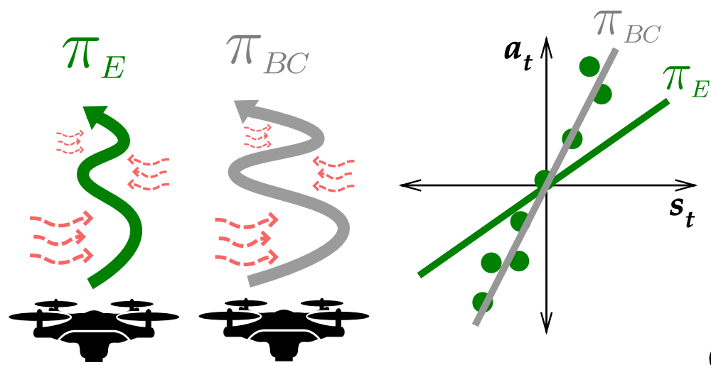
The first problem we’ll consider is when there’s temporally correlated noise (TCN) affecting pairs of expert actions. For example, if our expert was a human quadcopter pilot, the TCN could be persistent wind [1]. Let’s assume that the expert intended to fly completely straight but was unable to do so because of the persistent wind, producing swerving trajectories. If the learner ignores the fact that the wind was the root cause of these swerves, they might attempt to reproduce the swerving behavior of the expert, causing them to deviate even further at test time due to the continued influence of the wind.

What’s happened is that the TCN has created a spurious correlation (e.g. being a little on the left is often followed by going more to the left) which the learner has latched onto. What we’d like is to instead learn a policy that can fly as straight as the expert did in the demonstrations.

Let’s try and formalize what’s happening in the above example via graphical models. In a Markov Decision Process (MDP), the learner responds to the observed state via taking an action and the MDP transitions via dynamics to the next state .

Adding in the TCN corresponds to adding in a common cause of a pair of actions that’s not part of the observed state ( below).

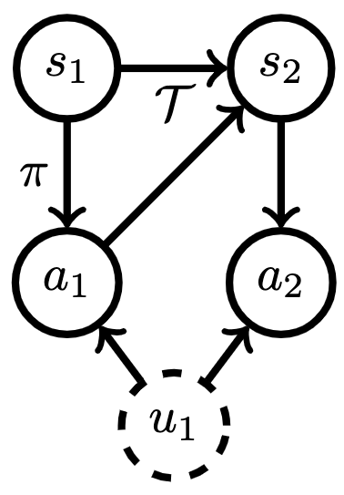
Now, let’s dig into what goes wrong with imitation learning under TCN. Let’s say we apply a standard algorithm like behavioral cloning: direct regression from states () to actions (). The TCN travels through the dynamics to influence both the inputs and outputs of our regression procedure, creating spurious correlations that our learner might latch onto, leading to poor test-time performance. We visualize this effect in red below.

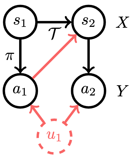
In effect, the TCN makes some elements of state look more correlated with action than they would otherwise. Attempting to minimize training error, the learner will use this correlation to their advantage but will end up swerving unnecessarily at test time as a result.

Filtering out TCN with instrumental variable regression

To learn well under TCN, we’re going to utilize the idea of a natural experiment from causal inference, in which we’re able to use variation in the observational data to simulate the effect of an intervention / randomized control trial (RCT). Interestingly enough, this idea was one of the central contributions of the winners of the Nobel Prize in Economics in 2021. Let’s first take a look at this idea in the single shot setting. Assume that we’re trying to predict from to , both of which are affected by an unobserved confounder :

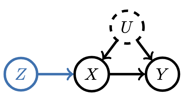
Notice the random variable both (1) affects and (2) is independent from . is therefore an independent source of variation in . We call such variables instruments. Under some assumptions (see our paper for details), one can condition on an instrument to de-noise the inputs to our regression procedure and recover a causal relationship. So, instead of regressing from

one regresses from

We’ll skip the derivation here but intuitively, conditioning on an independent source of variation, , “washes out” the effect of the confounder, . The variation in therefore acts as a sort of “natural experiment,” simulating an RCT without requiring a true intervention.

Now, you might well be wondering what a valid instrument in the sequential setting is? Well, given the past is independent of future confounding, we can use past states as an instrument! Graphically,

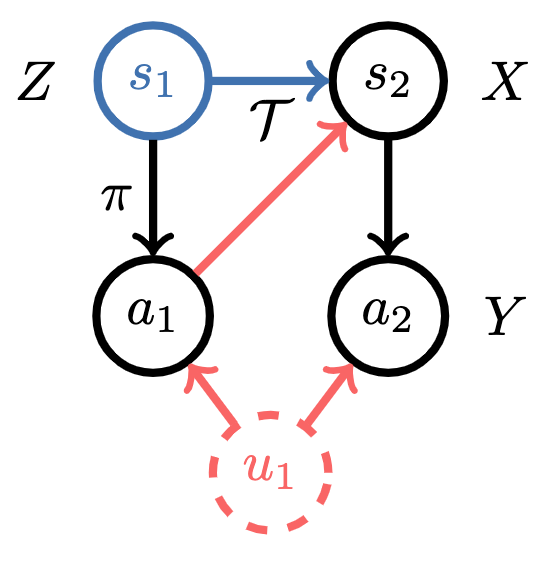
Many econometrics papers will spend quite a lot of text arguing something is a valid instrument (i.e. satisfies (1) and (2)) but here, the arrow of time gives us an instrument for free. Algorithmically, instrumental variable regression for imitation learning under TCN corresponds to solving

So, one first fits models of the left and right-hand sides of the above expression and then regresses between them. We give two algorithms for doing so efficiently in our paper. On simulated control tasks, we observe that our approaches (in teal and orange) are able to recover a policy that matches expert performance, while regression-based behavioral cloning struggles to do so.

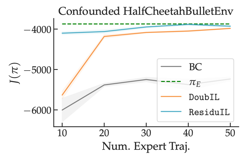
So, putting it all together, temporally correlated noise between expert actions can create spurious correlations between recorded states and actions, causing standard regression-based imitation learning approaches to produce inaccurate predictors. One can use the “natural experiment” caused by the variation in past states to de-noise the inputs to their regression procedure and recover causally correct predictors that do not suffer from spurious correlations.

Issue 2: Unobserved contexts

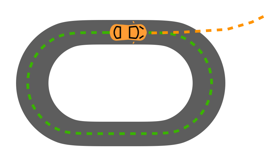
We’re now going to consider a different kind of confounder. Let’s assume we’re trying to imitate an expert who observes some context, , which the learner does not. For example, if we were trying to imitate an expert driver but our sensors don’t pick up a stop sign on the side of the road, could refer to this side information. Now, this problem is in general impossible to solve: if we don’t see the sign, how would we know to stop? However, if we pay attention to our surroundings and accumulate information over time, we might be able to eventually filter out what we missed: if we observe all the other cars around us slowing down for a few timesteps, we might rationally conclude that we should as well, even though we never saw the stop sign.

More formally, we’re in a Partially Observed Markov Decision Process (a POMDP), which we can visualize as follows:

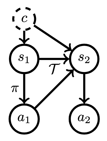
So, the effect of the stop sign () is reflected in the states (). There’s two key differences between this graphical model and the TCN graphical model. First, the confounder directly affects the state. Second, the confounder is constant, rather than time-varying. These two characteristics make it plausible that, given enough state observations, we can figure out what is and act as the expert does.

To enable us to accumulate evidence over time, we’re going to allow our policy to condition its actions on the entire history up to this point. Denoting , our policy now takes the form

This means our policy is now a sequence model (e.g. an RNN or a transformer).

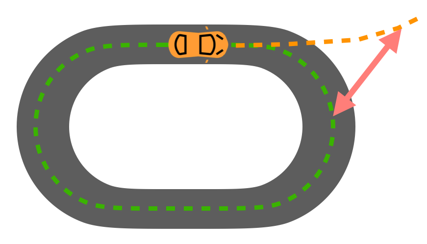
Ok, we use sequence models as our policy class and apply behavioral cloning (prediction of the next token from the prefix) and call it a day right? Unfortunately, this often produces policies that naively repeat their own past actions. We call this the latching effect. For example, in the self-driving domain, this can lead to learning a driving policy that begins to turn and then just keeps turning, driving in circles [2]. This is clearly less than ideal.

Modeling unobserved contexts with sequence models + on-policy training

Let’s dig into why the latching effect stymies off-policy imitation learners. The model we learn during training looks like

where the superscript denotes that these are expert states and actions. Now at test time, the past actions we pass into our sequence model policy are our own rather than the expert’s. This means we’re trying to sample actions from

Unless we know that the elements to the right of the conditioning bar are exactly the same (i.e. we’ve perfectly matched the expert policy), we have no reason to believe that the model we’ve learned will generalize to our own induced state distribution. Put differently, we have no reason to believe we’ve learned a policy which will perform well at test-time.

In machine learning terms, we’re facing the problem of policy-induced covariate shift (PICS). Here, our covariates are the history of states and actions the policy uses to predict the next action. PICS is a well known problem in imitation learning and sequential prediction writ large (see last blog post for more details). What’s special about the unobserved context setting is the degree to which it causes problems. Early on in an episode, no learner can do well as they haven’t accumulated enough information to perform well. This means that we have an unavoidable source of covariate shift from preliminary mistakes.

Now, let’s assume that the expert’s actions were relatively similar between adjacent timesteps (which is frequently true in practice). This means rather than learning a complex mapping from states to actions, our learner might have instead learned a policy that mostly copies the last action. This was fine when the previous actions were the expert’s. But when they are the learner’s extremely suboptimal initial actions, naive copying is a recipe for disaster. This is what leads to us learning a driving policy that is only capable of turning in circles. A different way of phrasing this point is because the learner was trained only on trajectories from the expert, it treats its own test-time past actions as though they were produced by the expert, leading to unfortunate downstream consequences.

On-policy training (i.e. performing rollouts in the environment and comparing them to expert rollouts) doesn’t suffer from these issues. This is because we’re instead trying to satisfy

In words, rather than matching expert actions on expert histories, we’re instead trying to match expert and learner trajectory distributions. We’re making sure we predict well based on our own histories and therefore can’t be surprised at test-time by states we didn’t expect to end up in. We prove in our paper that under certain identifiability conditions, on-policy training of sequence model policies is both necessary and sufficient for the learner to generalize well to their own induced state distribution and successfully imitate the expert.

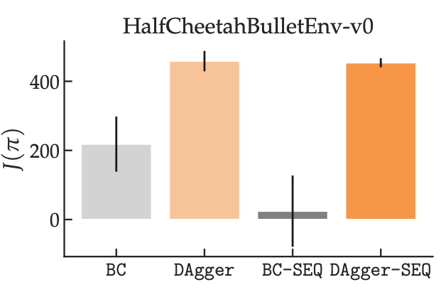
We also conduct experiments on continuous control tasks with unobserved contexts and show that equipping an off-policy learner (in grey) with access to history can actually hurt its performance, while we see no such effect for an on-policy learner (in orange).

Discussion

Confounding commonly occurs in real world situations, including those in which we want to make a sequence of decisions. When we don’t filter out or model the effects of what we don’t observe, we can end up making extremely suboptimal decisions. We describe two situations in which there’s clean algorithms for handling confounding in sequential decision making (temporally correlated noise can be filtered out via IVR, unobserved contexts can be modeled via on-policy training of a sequence model). Moving forward, we’re interested in other causal structures (e.g. negative controls or proxy shifts) and applying our techniques to problems where confounders abound (e.g. recommender systems).

If you’re interested in learning more, I recommend you look at the full papers or the attached code:

• The TCN Paper: Causal Imitation under Temporally Correlated Noise
• The TCN Code: https://github.com/gkswamy98/causal_il
• The Unobserved Contexts Paper: Sequence Model Imitation Learning with Unobserved Contexts
• The Unobserved Contexts Code: https://github.com/gkswamy98/sequence_model_il

DISCLAIMER: All opinions expressed in this post are those of the author and do not represent the views of CMU.

This article was initially published on the ML@CMU blog and appears here with the authors’ permission.

ML@CMU

ML@CMU