ΑΙhub.org
Universal weakly supervised segmentation by pixel-to-segment contrastive learning
By Tsung-Wei Ke and Jyh-Jing Hwang and Stella X. Yu
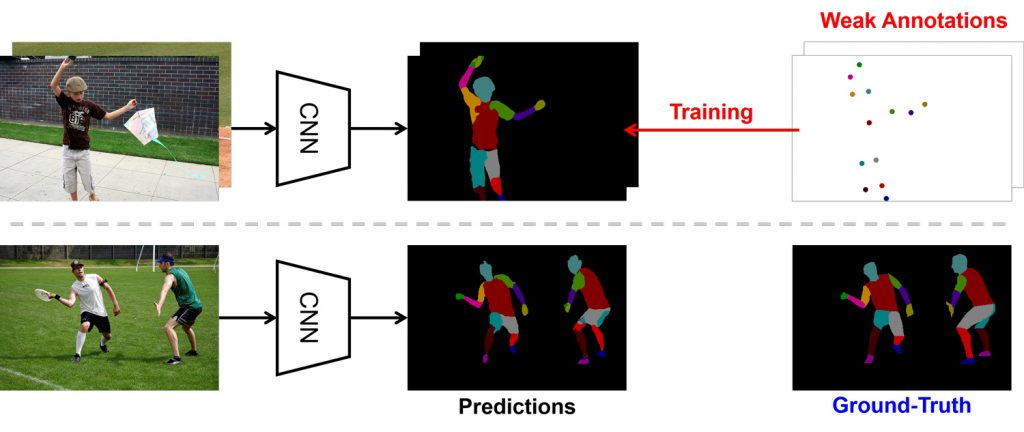
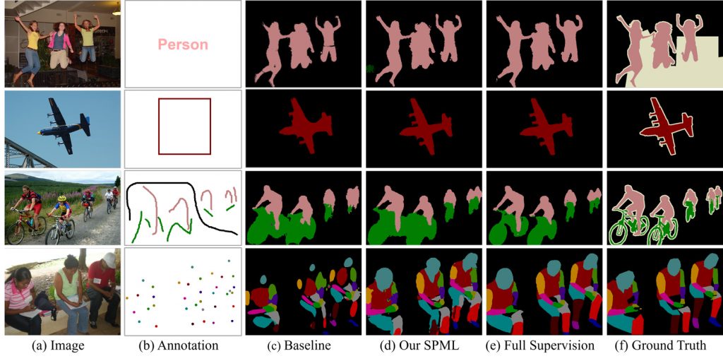
We consider a problem: Can a machine learn from a few labeled pixels to predict every pixel in a new image? This task is extremely challenging (see Fig. 1) as a single body part could contain visually distinctive areas (e.g. head consists of eyes, noses and mouths); different body parts might look similar and undistinguishable (e.g., upper arms v.s. lower arms). It could be even more difficult if we do not provide any precise location but only the occurrence of body parts in the image. This problem is dubbed weakly-supervised segmentation, where the goal is to classify every pixel into semantic categories using only partial / weak supervision. There are many forms of weak annotations which are cheap but not perfect, e.g. image-level tags, bounding boxes, points and scribbles.

These forms of weak supervision come with different assumptions and state-of-the-art methods tackle them differently. Weak supervision can be roughly categorized into two families: Coarse and Sparse supervision. Coarse annotations, including image tags and bounding boxes, lack precise pixel localization and rely on Class Activation Map (CAM) to localize coarse semantic cues and generate pseudo pixel labels. Sparse annotations, such as points and scribbles, only label a small subset of pixels and Conditional Random Fields (CRF) are often used to propagate labels to unlabeled pixels. However, it is frustrating to develop individual methods for each form of weak supervision. This problem motivates us to develop a single method to deal with universal weakly supervised segmentation problems. In fact, weakly supervised segmentation problems can be regarded as semi-supervised pixel classification problems. And the key is how to propagate and refine annotations from coarsely and sparsely labeled pixels to unlabeled pixels?
Metric learning and contrastive loss formulation
To solve the semi-supervised learning problem, we take the viewpoint of feature representation learning. We aim at learning the most optimal pixel-wise feature mapping to group (separate) pixels of the same (different) category. For every pixel in the image, we generate corresponding embeddings (or feature representations) using a segmentation CNN. We thus can propagate the semantic labels from labeled pixels to neighboring unlabeled ones in this latent feature space.
We adopt a metric learning framework and contrastive loss formulation to learn the optimal pixel-wise feature mapping. More specifically, we break down an image into several segments and compute the representative features for each segment (by averaging pixel embeddings within each segment). For each pixel, we collect same-category segments as the positive set, and vice versa. As shown in the following figure, we then train the network to increase (decrease) the distance between the pixel and its positive (negative) set of segments.

Grouping relationships from weak supervision
Here, we see a problem immediately emerging in the metric learning framework. How do we deal with unlabeled pixels and segments in the metric learning framework? Under the supervised setting, unlabeled pixels and segments are ignored in the contrastive loss formulation. In the case of point annotations, as most pixels are unlabeled, the supervision signal will be too sparse to learn a good feature mapping.
Instead, our key insight is to integrate them into discriminative feature learning to strengthen the supervision. We explore four grouping relationships derived from visual cues and semantic information in images. According to these grouping relationships, we can define corresponding positive and negative sets for every pixel in the image. As shown in the following figure, the grouping relationships are based on (a) low-level image similarity, (b) semantic annotations, (c) semantic co-occurrence and (d) feature affinity.
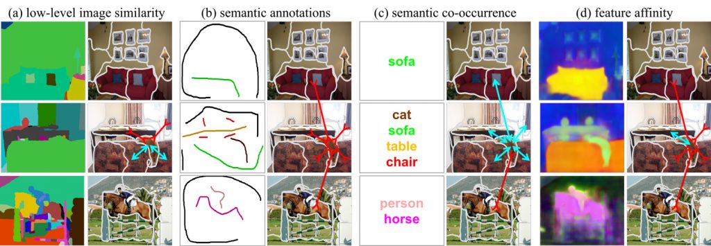
In fact, each grouping relationship corresponds to a specific prior, which is introduced as one of the learning objectives for the pixel-wise feature mapping. (a) low-level image similarity correlates with a spatial smoothness prior in visually coherent regions. The intuition is that pixels of similar appearance are more likely to be in the same category. (b) semantic annotations are the localized semantic cues in the image, such as points / scribbles / CAMs. (c) semantic co-occurrence reflects scene-context similarity. Objects in the same scene should be more semantically similar than the ones in different scenes. For example, wildlife animals are always outdoor, but furniture is usually indoor. We consider two images sharing any of semantic classes as similar-context, and vice versa. (d) feature affinity considers smoothness prior in the latent feature space.
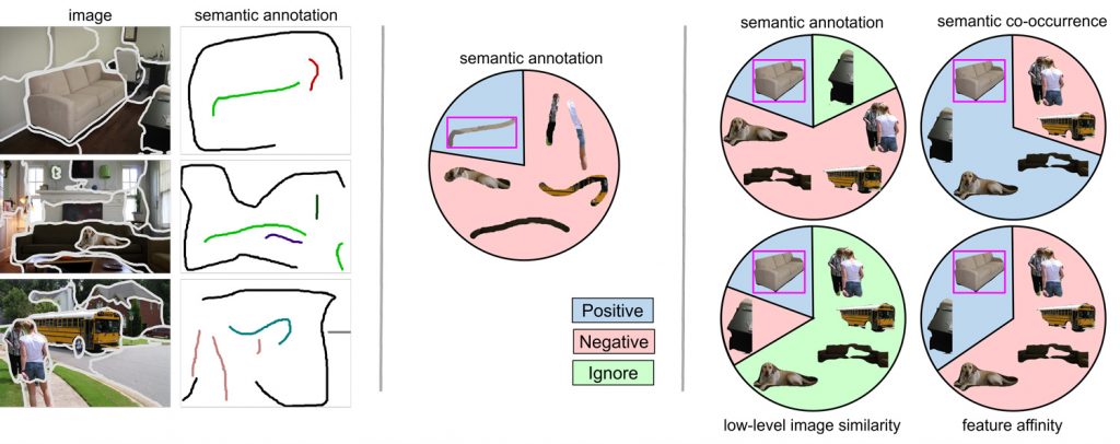
As shown in the figure above, we can define corresponding positive and negative sets of segments, and derive four contrastive losses w.r.t each grouping relationship. By training the segmentation CNN with these losses jointly, we can find the most optimal feature mapping.
Across-the-board improvements
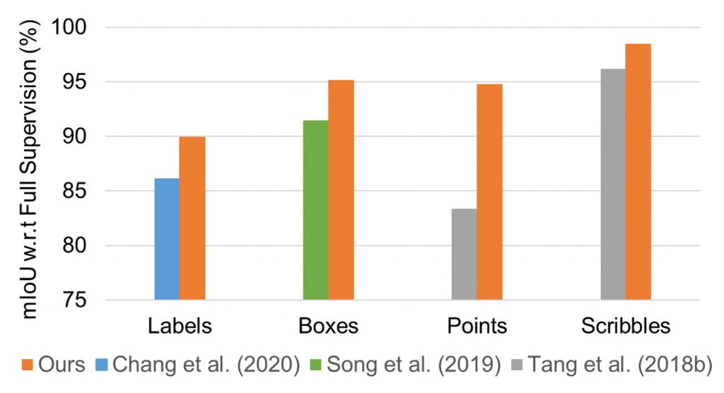
As demonstrated in the following figures, our approach outperforms other methods by large margin for every form of weak supervision.
Contextual retrievals
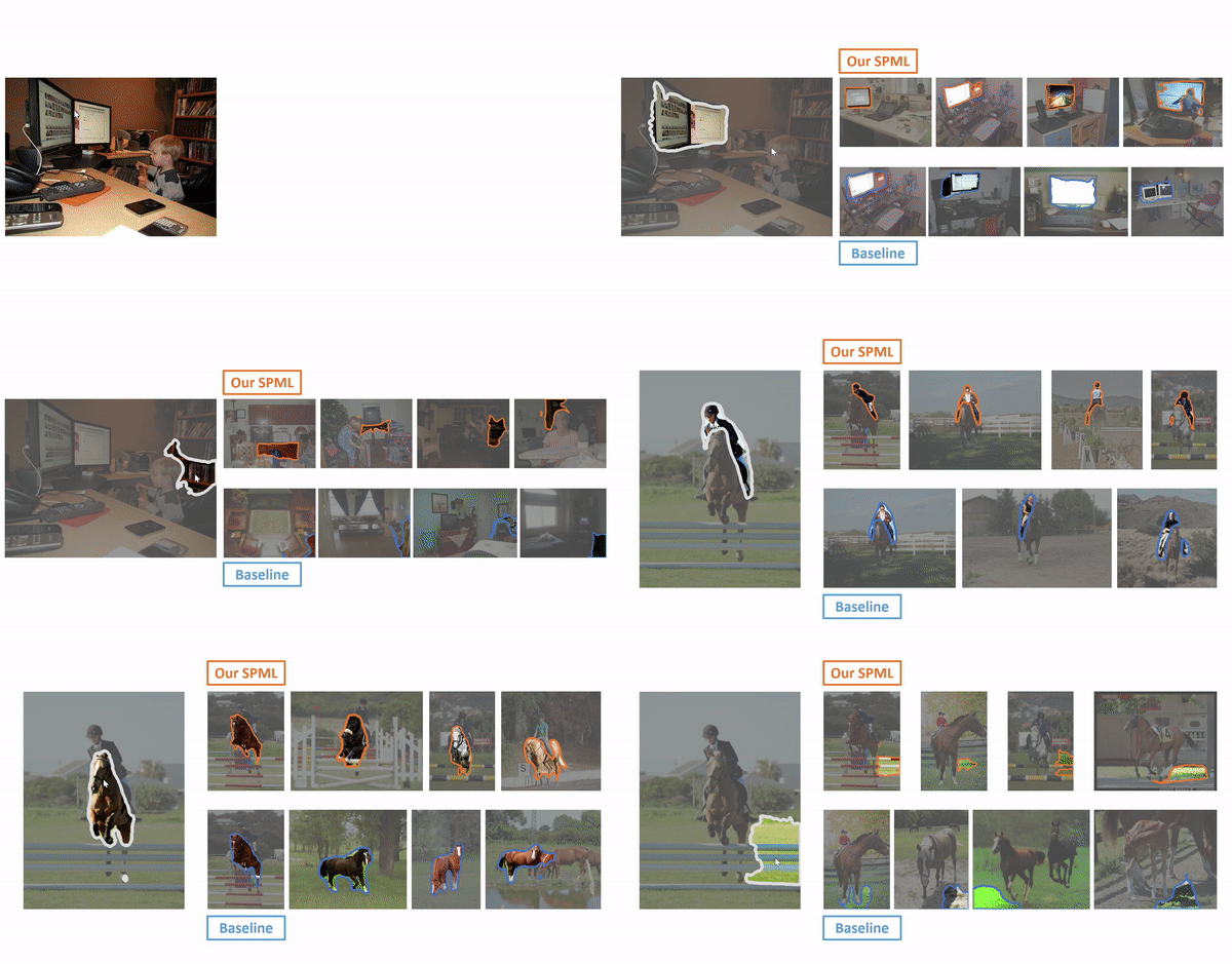
To demonstrate the semantic information encoded by pixel-wise feature mapping, we perform nearest neighbor retrievals using the image segments and their features. As shown in the following figure, given the query segment (left), we observe our retrievals (top right) are in a more similar scene context than baseline method (bottom right). For example, our retrieved horses are jumping over hurdles, which matches the context of the query horse.
A solution for universal weakly supervised segmentation
In this work, we propose a single method to tackle all forms of weak supervision, even if they carry different assumptions. Our core idea is to learn the pixel-wise feature mapping, which respects various types of grouping relationships. These grouping relationships can be easily derived from low-level visual cues and semantic information in images. Lastly, we demonstrate superior performance over other baseline methods given every form of weak annotations.
We thank all co-authors of the paper “Universal Weakly Supervised Segmentation by Pixel-to-Segment Contrastive Learning” for their contributions and insights for preparing this blog. The paper is presented at ICLR 2021. You can see results on our website, and we provide code to to reproduce our experiments.
This article was initially published on the BAIR blog, and appears here with the authors’ permission.
tags: deep dive
