Riemannian score-based generative modelling

By Valentin De Bortoli, Emile Mathieu, Michael Hutchinson, James Thornton, Yee Whye Teh and Arnaud Doucet

From protein design to machine learning

How can machine learning help us synthesize new proteins with specific properties and behaviour? Coming up with efficient, reliable and fast algorithms for protein synthesis would be transformative for areas such as vaccine design. This is one of many questions that generative modelling tries to answer. But first, what is generative modelling? In a few words, it is the task of obtaining samples from an unknown data distribution . Of course, one has to assume some knowledge of this target distribution . In statistical science, we usually assume that we have access to an unnormalised density such that . In machine learning, we take a different approach and only assume that we know through a collection of samples. In our running example of protein design, we assume that we have access to a collection of proteins (for example via the Protein Data Bank, PDB [1].

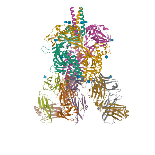Figure 1: One of the many proteins available on PDB. Here, the crystal structure of the Nipah virus fusion glycoprotein (id-6T3F), see [2].

Once we have this set of examples (called the training dataset) our goal is to come up with an algorithm to obtain samples that are distributed similarly to the training dataset, i.e. samples from .

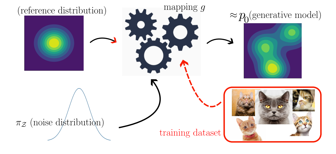Figure 2: An illustrative picture of modern machine learning generative modelling. We draw samples from a reference probability distribution and then modify these samples using a learnable function (which might be stochastic). The output samples are close to the true distribution .

There exists a myriad of generative models out there, to cite a few: Variational AutoEncoders (VAEs) [13], Generative Adversarial Networks (GANs) [4], Normalizing Flows (NF) [20] and the latest newcomer, Diffusion Models [26, 6, 27]. Diffusion Models were introduced in late 2019 (based on earlier work on Nonequilibrium Thermodynamics [25]). This new class of generative models has seen impressive success in synthesising images with the most stunning applications being a flurry of text-to-image models like DALL.E-2 [19] Imagen [24], Midjourney [16] or Stable Diffusion [22].

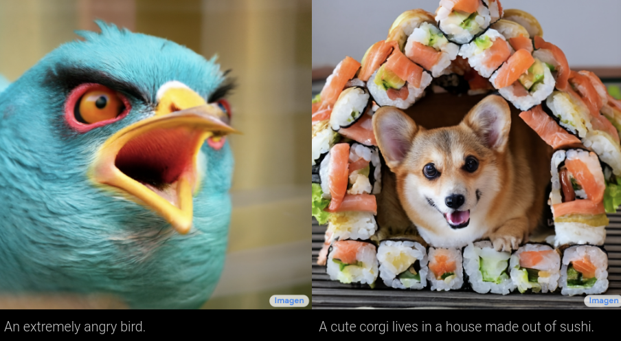Figure 3: Samples from the text-to-image model Imagen [24].

It’s a Riemannian world. One key advantage of Diffusion Models over existing methods is their flexibility. For instance, Diffusion Models have also been applied to obtain state-of-the-art (SOTA) results in text-to-audio [21], text-to-3D [18], conditional and unconditional video generation [7]. Hence, one can wonder if the underlying principles of Diffusion Models can also be used in the context of protein design. In order to understand how we can adapt Diffusion Models to this challenging task, we need to take a quick detour and first describe the type of data we are dealing with. In the case of video, audio and shape, the samples are elements of a Euclidean space for some , for example in the case of a RGB image. The case of proteins, however, is a little bit more involved. A protein is comprised of a sequence of amino-acids (parameterised by atoms ) with a particular arrangement in the three-dimensional space. Hence, a good first guess to parameterise the data is to work in the space , where is the length of the amino-acid sequence [29]. In that case we only model the position of the atom in each amino-acid. Unfortunately, this is not enough if one wants to precisely describe the fine-grained structure (secondary and tertiary structure) of the protein. Indeed, we need to also consider the position of the atoms¹ , . Due to biochemical constraints, the relative positive positions of these atoms to is only described by a rotation, describing the intrisic pose of the amino-acid. Doing so the data is not supported on but on , where is the space of rigid motions (combinations of rotations and translations) [12].

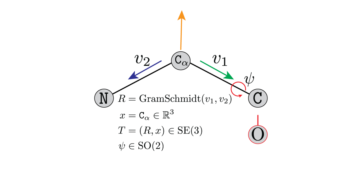Figure 4: A rotation matrix parameterises the . The atom is at position . An additional torsion angle, , is required to determine the placement of the oxygen atom . parameterise the amino-acid. Credit to Brian Trippe and Jason Yim for the image.

However, we are now outside of the comfort zone of Euclidean data and enter the realm of Riemannian geometry. Indeed the space , and by extension , is not a vector space anymore but a manifold, i.e. a space that resembles to a Euclidean space only locally. The manifold is said to be Riemannian if we can endow it with a notion of distance. Some examples of Riemannian manifolds include the sphere in , the group of rotations or the Poincaré ball. The tools developed for Diffusion Models cannot be directly applied to the Riemannian setting. The goal of our paper “Riemannian Score-Based Generative Modelling” [3] is to extend the ideas and techniques of Diffusion Models to this more general setting. Note that the applications of Riemannian generative modelling include but are not restricted to protein design applications. Indeed, similar challenges arise when trying to model admissible movements in robotics or when studying geoscience data.

The rise of diffusion models. Before diving into the core of our contribution, we start by recalling the main ideas underlying Diffusion Models. Very briefly Diffusion Models consist in 1) a forward process progressively adding noise to the data, destroying the information and converging on a reference distribution 2) a backward process which gradually reverts the forward model starting from the reference distribution. The output of the backward process is our generative model. In practice, the forward noising process is given by a Stochastic Differential Equation (SDE)

(1)  

where is a Brownian motion. In layman terms, this means that starting from , the next point is obtained via

(2)  

where is a Gaussian random variable and . It can be shown that such a process converges exponentially fast to . Of course, this is the easy part, there exist, after all, many ways to destroy the data. It turns out that when the destroying process is described via this SDE framework there exists another SDE describing the same process run backward in time. Namely, putting

(3)  

with initial condition , we have that as the same distribution as [5]. There we have it. The output of this SDE is our generative model. Of course in order to compute this SDE and propagate we need to initialise and compute (where is the density of ). In the statistics literature is called the score. This is a vector field pointing in the direction with the most density.

Figure 5: The evolution of particles following the Langevin dynamics targeting a mixture of Gaussians with distribution . Black arrows represent the score . Credit: Yang Song.

It turns out that is untractable but can be efficiently estimated using tools from score-matching. Namely, one can find a tractable loss function whose minimiser is the score. Hence, the training part of Diffusion Models consists of learning this score function. Once this done we approximately sample from the associated SDE by computing

(4)  

where is the score approximation of (usually given by a U-net, although things are changing [17, 10]). To initialize , we simply sample from a Gaussian distribution since this distribution is close to the one of .

Figure 6: Evolution of the dynamics , starting from a Gaussian distribution and targeting a data distribution . Credit: Yang Song.

From Euclidean to Riemannian. With this primer on Diffusion models in Euclidean spaces, we are now ready to extend them to Riemannian manifolds. First, it is important to emphasise how much the classical presentation of Diffusion Models is dependent on the Euclidean structure of the space. For example, it does not make sense to talk about a Gaussian random variable on the sphere or on the space of rotations (even though equivalent notions can be defined but we will come to that in a moment). Similarly, the discretisation of the SDE we presented is called the Euler-Maruyama discretisation and only makes sense in Euclidean spaces (what does the operator mean on the sphere?). In our work we identify four main ingredients which are sufficient and necessary to define a Diffusion Model in an arbitrary space:
(a) A forward noising process.
(b) A backward denoising process.
(c) An algorithm to (approximately) sample from these processes.
(d) A toolbox for the approximation of extension of score functions.

It turns out that SDEs can also be defined on Riemannian manifolds under reasonable conditions on the geometry. More precisely, as long as one can define a notion of metric (which is required when considering Riemannian manifolds) we can make sense of the equation

(5)  

for a potential defined on the manifold. However, we need to replace the notion of gradient with the one of Riemannian gradient which is dependent on the metric (we refer to [14] for a rigorous treatment of these notions). In the special case where the Riemannian manifold is compact one can set and then the process becomes the Brownian motion and converges towards the uniform distribution.

Once we have defined our forward process, we still need to consider its time-reversal as in the Euclidean setting. In the previous setting, we could use a formula to deduce the backward process from the forward process. It turns out that this formula is still true in the Riemannian setting! This is provided that the notion of gradient in the score term is replaced with the one Riemannian gradient.

So far so good, we can define forward and backward processes to sample from the target distribution. However, in practice we need a Riemannian equivalent of the Euler-Maruyama (EM) discretisation to obtain a practical algorithm. To do so, we use what is called the Geodesic Random Walk [11] which coincides with EM in the Euclidean setting. It replaces the operator in the Euler-Maruyama discretisation by the exponential mapping on the manifold.

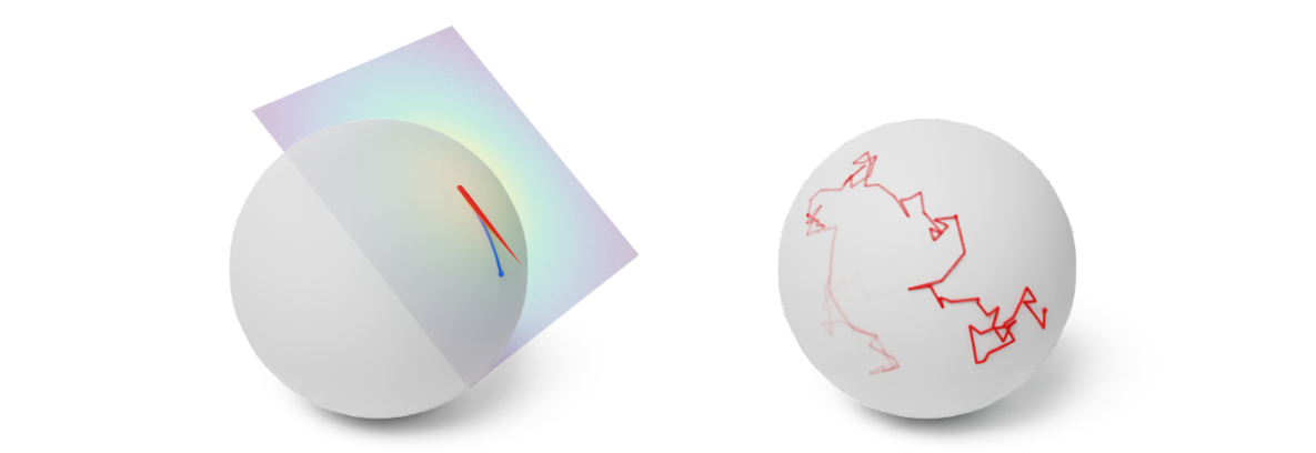Figure 7: (Left) One step of the Geodesic Random Walk with perturbation in the tangent space. (Right) Many steps of the Geodesic Random Walk yield an approximate Brownian motion trajectory. Credit: Michael Hutchinson.

For example

(6)  

becomes

(7)  

where computes the geodesics on the manifold, i.e. the length-minimizing curve starting from and direction . Finally, it is easy to show that the Euclidean score-matching loss can be extended to the Riemannian setting by replacing all references to the Euclidean metric by the Riemannian metric.

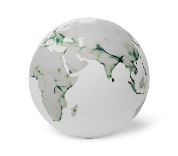
Once these tools are in place we are ready to implement Diffusion Models on Riemannian manifolds. In our work, we present toy examples on the sphere and as well as geoscience data and model the distribution of volcanoes, earthquakes, floods and fires on Earth. We show that our model achieves SOTA likelihood results when compared to its Normalizing Flow inspired competitor [23].

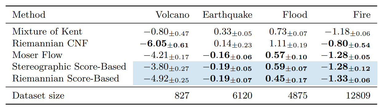Table 1: Negative log-likelihood scores for each method on the earth and climate science datasets. Bold indicates best results (up to statistical significance). Means and confidence intervals are computed over 5 different runs. Novel methods are shown with blue shading.

In particular, one striking feature of Diffusion Models is their robustness with respect to the dimension. We show that these models can still achieve good performance in dimension while other methods fail. We emphasise that since our work, several improvements have been proposed building on the Riemannian Diffusion Models framework [8, 28].

Figure 8: Evolution of the backward dynamics targeting the Dirac mass on the sphere. Credit: Michael Hutchinson.

What lies beyond. This work introduces a framework for principled diffusion-based generative modelling for Riemannian data. As emphasised in the introduction, one key application of such models is protein design. Since then there has been a flurry of work using or diffusion models to synthesise new proteins with impressive results [9, 30]. In particular, [30] uses the flexibility of the diffusion models to impose structural constraints on the protein (such as some cyclical invariance to generate a trimer for example) or to minimise additional loss functions. Our work also opens the door to several generalisations of Diffusion models to Lie groups (such as for lattice Quantum ChromoDynamics applications [1]) using the special structure of these manifolds. Finally, as of now, we require some knowledge on the manifold in order to incorporate this geometric information in our generative model (exponential mapping, metric, parameterisation). However, while it is customary to make the assumption that the data is supported on a manifold in applications such as image modelling, the manifold of interest is not known and is discovered during the generation procedure, as in [15]. It is still an open problem to investigate how this partial information can be incorporated in a Riemannian generative model.

References

[1] Albergo, M. S., Boyda, D., Hackett, D. C., Kanwar, G., Cranmer, K., Racani`ere, S., Rezende, D. J., and Shanahan, P. E. (2021). Introduction to normalizing flows for lattice field theory. arXiv preprint arXiv:2101.08176.
[2] Avanzato, V. A., Oguntuyo, K. Y., Escalera-Zamudio, M., Gutierrez, B., Golden, M., Kosakovsky Pond, S. L., Pryce, R., Walter, T. S., Seow, J., Doores, K. J., et al. (2019). A structural basis for antibody-mediated neutralization of nipah virus reveals a site of vulnerability at the fusion glycoprotein apex. Proceedings of the National Academy of Sciences, 116(50):25057–25067.
[3] De Bortoli, V., Mathieu, E., Hutchinson, M., Thornton, J., Teh, Y. W., and Doucet, A. (2022). Riemannian score-based generative modeling. arXiv preprint arXiv:2202.02763.
[4] Goodfellow, I. J., Pouget-Abadie, J., Mirza, M., Xu, B., Warde-Farley, D., Ozair, S., Courville, A., and Bengio, Y. (2014). Generative adversarial networks. arXiv preprint arXiv:1406.2661.
[5] Haussmann, U. G. and Pardoux, E. (1986). Time reversal of diffusions. The Annals of Probability, 14(4):1188–1205.
[6] Ho, J., Jain, A., and Abbeel, P. (2020). Denoising diffusion probabilistic models. Advances in Neural Information Processing Systems.
[7] Ho, J., Salimans, T., Gritsenko, A., Chan, W., Norouzi, M., and Fleet, D. J. (2022). Video diffusion models. arXiv preprint arXiv:2204.03458.
[8] Huang, C.-W., Aghajohari, M., Bose, A. J., Panangaden, P., and Courville, A. (2022). Riemannian diffusion models. arXiv preprint arXiv:2208.07949.
[9] Ingraham, J., Baranov, M., Costello, Z., Frappier, V., Ismail, A., Tie, S., Wang, W., Xue, V., Obermeyer, F., Beam, A., et al. (2022). Illuminating protein space with a programmable generative model. bioRxiv.
[10] Jabri, A., Fleet, D., and Chen, T. (2022). Scalable adaptive computation for iterative generation. arXiv preprint arXiv:2212.11972.
[11] Jørgensen, E. (1975). The central limit problem for geodesic random walks. Zeitschrift für Wahrscheinlichkeitstheorie und verwandte Gebiete, 32(1):1–64.
[12] Jumper, J., Evans, R., Pritzel, A., Green, T., Figurnov, M., Ronneberger, O., Tunyasuvunakool, K., Bates, R., Žídek, A., Potapenko, A., et al. (2021). Highly accurate protein structure prediction with alphafold. Nature, 596(7873):583–589.
[13] Kingma, D. P. and Welling, M. (2013). Auto-encoding variational bayes. arXiv preprint arXiv:1312.6114.
[14] Lee, J. M. (2018). Introduction to Riemannian manifolds, volume 176. Springer.
[15] Lou, A., Nickel, M., Mukadam, M., and Amos, B. (2021). Learning complex geometric structures from data with deep riemannian manifolds.
[16] Midjourney (2022). https://midjourney.com/.
[17] Peebles, W. and Xie, S. (2022). Scalable diffusion models with transformers. arXiv preprint arXiv:2212.09748.
[18] Poole, B., Jain, A., Barron, J. T., and Mildenhall, B. (2022). Dreamfusion: Text-to-3d using 2d diffusion. arXiv preprint arXiv:2209.14988.
[19] Ramesh, A., Dhariwal, P., Nichol, A., Chu, C., and Chen, M. (2022). Hierarchical text-conditional image generation with clip latents. arXiv preprint arXiv:2204.06125.
[20] Rezende, D. and Mohamed, S. (2015). Variational inference with normalizing flows. In International conference on machine learning, pages 1530–1538. PMLR.
[21] Riffusion (2022). https://www.riffusion.com/.
[22] Rombach, R., Blattmann, A., Lorenz, D., Esser, P., and Ommer, B. (2022). High-resolution image synthesis with latent diffusion models. In Proceedings of the IEEE/CVF Conference on Computer Vision and Pattern Recognition, pages 10684–10695.
[23] Rozen, N., Grover, A., Nickel, M., and Lipman, Y. (2021). Moser flow: Divergence-based generative modeling on manifolds. Advances in Neural Information Processing Systems, 34:17669–17680.
[24] Saharia, C., Chan, W., Saxena, S., Li, L., Whang, J., Denton, E., Ghasemipour, S. K. S., Ayan, B. K., Mahdavi, S. S., Lopes, R. G., et al. (2022). Photorealistic text-to-image diffusion models with deep language understanding. arXiv preprint arXiv:2205.11487.
[25] Sohl-Dickstein, J., Weiss, E., Maheswaranathan, N., and Ganguli, S. (2015). Deep unsupervised learning using nonequilibrium thermodynamics. In International Conference on Machine Learning.
[26] Song, Y. and Ermon, S. (2019). Generative modeling by estimating gradients of the data distribution. In Advances in Neural Information Processing Systems.
[27] Song, Y., Sohl-Dickstein, J., Kingma, D. P., Kumar, A., Ermon, S., and Poole, B. (2021). Score-based generative modeling through stochastic differential equations. In International Conference on Learning Representations.
[28] Thornton, J., Hutchinson, M., Mathieu, E., De Bortoli, V., Teh, Y. W., and Doucet, A. (2022). Riemannian diffusion schrödinger bridge. arXiv preprint arXiv:2207.03024.
[29] Trippe, B. L., Yim, J., Tischer, D., Broderick, T., Baker, D., Barzilay, R., and Jaakkola, T. (2022). Diffusion probabilistic modeling of protein backbones in 3d for the motif-scaffolding problem. arXiv preprint arXiv:2206.04119.
[30] Watson, J. L., Juergens, D., Bennett, N. R., Trippe, B. L., Yim, J., Eisenach, H. E., Ahern, W., Borst, A. J., Ragotte, R. J., Milles, L. F., et al. (2022). Broadly applicable and accurate protein design by integrating structure prediction networks and diffusion generative models. bioRxiv.

¹To obtain a proper end-to-end protein model one also needs to design a generative model to predict , usually given by a element of . For simplicity, we omit this step.

Valentin De Bortoli is a research scientist at CNRS and the Center for Data Science in Ecole Normale Supérieure in Paris.

Valentin De Bortoli is a research scientist at CNRS and the Center for Data Science in Ecole Normale Supérieure in Paris.